Developing solvers with Red Hat Build of OptaPlanner
Abstract
Preface
You can use Red Hat Build of OptaPlanner to develop solvers that determine the optimal solution to planning problems. OptaPlanner is a built-in component of Red Hat Build of OptaPlanner. You can use solvers as part of your services in Red Hat Build of OptaPlanner to optimize limited resources with specific constraints.
Making open source more inclusive
Red Hat is committed to replacing problematic language in our code, documentation, and web properties. We are beginning with these four terms: master, slave, blacklist, and whitelist. Because of the enormity of this endeavor, these changes will be implemented gradually over several upcoming releases. For more details, see our CTO Chris Wright’s message.
Part I. Release notes for Red Hat Build of OptaPlanner 8.38
These release notes list new features and provide upgrade instructions for Red Hat Build of OptaPlanner 8.38.
Chapter 1. Upgrading from OptaPlanner 8.13 to Red Hat Build of OptaPlanner 8.38
To upgrade from OptaPlanner 8.13 to Red Hat Build of OptaPlanner 8.38, merge the previous versions of OptaPlanner in the following order:
Procedure
- Open the OptaPlanner Upgrade Recipe 8 page in a browser.
- Complete the instructions for first version that you want to upgrade, for example From 8.13.0.Final to 8.14.0.Final.
- Repeat the instructions until you have upgraded to 8.37.0.Final.
Chapter 2. Red Hat Build of OptaPlanner 8.38 new features
This section highlights new features in Red Hat Build of OptaPlanner 8.38.
Bavet is a feature used for fast score calculation. Bavet is currently only available in the community version of OptaPlanner. It is not available in Red Hat Build of OptaPlanner 8.38.
2.1. Performance improvements in pillar moves and nearby selection
OptaPlanner can now auto-detect situations where multiple pillar move selectors can share a precomputed pillar cache and reuse it instead of recomputing the pillar cache for each move selector. If you combine pillar moves, for example, PillarChangeMove and PillarSwapMove, you should see significant performance inprovements.
This also applies if you use nearby selection. OptaPlanner can now auto-detect situations where a precomputed distance matrix can be shared between multiple move selectors, which saves memory and CPU processing time.
As a consequence of this enhancement, implementations of the following interfaces are expected to be stateless:
-
org.optaplanner.core.impl.heuristic.selector.common.nearby.NearbyDistanceMeter -
org.optaplanner.core.impl.heuristic.selector.common.decorator.SelectionFilter -
org.optaplanner.core.impl.heuristic.selector.common.decorator.SelectionProbabilityWeightFactory -
org.optaplanner.core.impl.heuristic.selector.common.decorator.SelectionSorter -
org.optaplanner.core.impl.heuristic.selector.common.decorator.SelectionSorterWeightFactory
In general, if solver configuration asks the user to implement an interface, the expectation is that the implementation will be stateless or not try to include an external state. With the these performance improvements, failing to follow this requirement will result in subtle bugs and score corruption because the solver will now reuse these instances as it sees fit.
2.2. OptaPlanner configuration improvement
Various configuration classes, such as EntitySelectorConfig and ValueSelectorConfig, contain new builder methods which make it easier to replace XML-based solver configuration with fluent Java code.
2.3. PlanningListVariable support for K-Opt moves
A new move selector for list variables, KOptListMoveSelector, has been added. KOptListMoveSelector selects a single entity, removes k edges from its route, and adds k new edges from the removed edges' endpoints. KOptListMoveSelector can help the solver escape local optima in vehicle routing problems.
2.4. SolutionManager support for updating shadow variables
SolutionManager (formerly ScoreManager) methods such as explain(solution) and update(solution) received a new overload with an extra argument, SolutionUpdatePolicy. This is useful for users who load their solutions from persistent storage (such as a relational database), where these solutions do not include the information carried by shadow variables or the score. By calling these new overloads and picking the right policy, OptaPlanner automatically computes values for all of the shadow variables in a solution or recalculates the score, or both.
Similarly, ProblemChangeDirector received a new method called updateShadowVariables(), so that you can update shadow variables on demand in real-time planning.
2.5. Value range auto-detection
In most cases, links between planning variables and value ranges can now be automatically detected. Therefore, @ValueRangeProvider no longer needs to provide an ID property. Likewise, planning variables no longer need to reference value range providers through the valueRangeProviderRefs property.
No code changes or configuration changes are required. Users who prefer clarity over brevity can continue to explicitly reference value range providers.
Part II. Getting started with Red Hat Build of OptaPlanner
As a business rules developer, you can use Red Hat Build of OptaPlanner to find the optimal solution to planning problems based on a set of limited resources and under specific constraints.
Use this document to start developing solvers with OptaPlanner.
Chapter 3. Introduction to Red Hat Build of OptaPlanner
OptaPlanner is a lightweight, embeddable planning engine that optimizes planning problems. It helps normal Java programmers solve planning problems efficiently, and it combines optimization heuristics and metaheuristics with very efficient score calculations.
For example, OptaPlanner helps solve various use cases:
- Employee/Patient Rosters: It helps create timetables for nurses and keeps track of patient bed management.
- Educational Timetables: It helps schedule lessons, courses, exams, and conference presentations.
- Shop Schedules: It tracks car assembly lines, machine queue planning, and workforce task planning.
- Cutting Stock: It minimizes waste by reducing the consumption of resources such as paper and steel.
Every organization faces planning problems; that is, they provide products and services with a limited set of constrained resources (employees, assets, time, and money).
OptaPlanner is open source software under the Apache Software License 2.0. It is 100% pure Java and runs on most Java virtual machines (JVMs).
3.1. Backwards compatibility
OptaPlanner separates the API and the implementation:
- Public API: All classes in the package namespace org.optaplanner.core.api, org.optaplanner.benchmark.api, org.optaplanner.test.api and org.optaplanner.persistence.api are 100% backwards compatible in future minor and patch releases. In rare instances, if the major version number changes, a few specific classes might have a few backwards incompatible changes, but those changes will be clearly documented in the upgrade recipe.
- XML configuration: The XML solver configuration is backwards compatible for all elements, except for elements that require the use of non-public API classes. The XML solver configuration is defined by the classes in the package namespace org.optaplanner.core.config and org.optaplanner.benchmark.config.
- Implementation classes: All other classes are not backwards compatible. They will change in future major or minor releases. The upgrade recipe describes relevant changes and on how to resolve them when upgrading to a newer version.
3.2. Planning problems
A planning problem has an optimal goal, based on limited resources and under specific constraints. Optimal goals can be any number of things, such as:
- Maximized profits - the optimal goal results in the highest possible profit.
- Minimized ecological footprint - the optimal goal has the least amount of environmental impact.
- Maximized satisfaction for employees or customers - the optimal goal prioritizes the needs of employees or customers.
The ability to achieve these goals relies on the number of resources available. For example, the following resources might be limited:
- Number of people
- Amount of time
- Budget
- Physical assets, for example, machinery, vehicles, computers, buildings
You must also take into account the specific constraints related to these resources, such as the number of hours a person works, their ability to use certain machines, or compatibility between pieces of equipment.
Red Hat Build of OptaPlanner helps Java programmers solve constraint satisfaction problems efficiently. It combines optimization heuristics and metaheuristics with efficient score calculation.
3.3. NP-completeness in planning problems
The provided use cases are probably NP-complete or NP-hard, which means the following statements apply:
- It is easy to verify a specific solution to a problem in reasonable time.
- There is no simple way to find the optimal solution of a problem in reasonable time.
The implication is that solving your problem is probably harder than you anticipated, because the two common techniques do not suffice:
- A brute force algorithm (even a more advanced variant) takes too long.
- A quick algorithm, for example in the bin packing problem, putting in the largest items first returns a solution that is far from optimal.
By using advanced optimization algorithms, OptaPlanner finds a good solution in reasonable time for such planning problems.
3.4. Solutions to planning problems
A planning problem has a number of solutions.
Several categories of solutions are:
- Possible solution
- A possible solution is any solution, whether or not it breaks any number of constraints. Planning problems often have an incredibly large number of possible solutions. Many of those solutions are not useful.
- Feasible solution
- A feasible solution is a solution that does not break any (negative) hard constraints. The number of feasible solutions are relative to the number of possible solutions. Sometimes there are no feasible solutions. Every feasible solution is a possible solution.
- Optimal solution
- Optimal solutions are the solutions with the highest scores. Planning problems usually have a few optimal solutions. They always have at least one optimal solution, even in the case that there are no feasible solutions and the optimal solution is not feasible.
- Best solution found
- The best solution is the solution with the highest score found by an implementation in a specified amount of time. The best solution found is likely to be feasible and, given enough time, it’s an optimal solution.
Counterintuitively, the number of possible solutions is huge (if calculated correctly), even with a small data set.
In the examples provided in the optaplanner-examples/src distribution folder, most instances have a large number of possible solutions. As there is no guaranteed way to find the optimal solution, any implementation is forced to evaluate at least a subset of all those possible solutions.
OptaPlanner supports several optimization algorithms to efficiently wade through that incredibly large number of possible solutions.
Depending on the use case, some optimization algorithms perform better than others, but it is impossible to know in advance. Using OptaPlanner, you can switch the optimization algorithm by changing the solver configuration in a few lines of XML or code.
3.5. Constraints on planning problems
Usually, a planning problem has minimum two levels of constraints:
A (negative) hard constraint must not be broken.
For example, one teacher can not teach two different lessons at the same time.
A (negative) soft constraint should not be broken if it can be avoided.
For example, Teacher A does not like to teach on Friday afternoons.
Some problems also have positive constraints:
A positive soft constraint (or reward) should be fulfilled if possible.
For example, Teacher B likes to teach on Monday mornings.
Some basic problems only have hard constraints. Some problems have three or more levels of constraints, for example, hard, medium, and soft constraints.
These constraints define the score calculation (otherwise known as the fitness function) of a planning problem. Each solution of a planning problem is graded with a score. With OptaPlanner, score constraints are written in an object oriented language such as Java, or in Drools rules.
This type of code is flexible and scalable.
3.6. Examples provided with Red Hat Build of OptaPlanner
Several OptaPlanner examples are shipped with Red Hat Build of OptaPlanner. You can review the code for examples and modify it as necessary to suit your needs.
Red Hat does not provide support for the example code included in the Red Hat Build of OptaPlanner distribution.
Some of the OptaPlanner examples solve problems that are presented in academic contests. The Contest column in the following table lists the contests. It also identifies an example as being either realistic or unrealistic for the purpose of a contest. A realistic contest is an official, independent contest that meets the following standards:
- Clearly defined real-world use cases
- Real-world constraints
- Multiple real-world datasets
- Reproducible results within a specific time limit on specific hardware
- Serious participation from the academic and/or enterprise Operations Research community.
Realistic contests provide an objective comparison of OptaPlanner with competitive software and academic research.
| Example | Domain | Size | Contest | Directory name |
|---|---|---|---|---|
| 1 entity class (1 variable) |
Entity ⇐
Value ⇐
Search space ⇐ | Pointless (cheatable) |
| |
| 1 entity class (1 variable) |
Entity ⇐
Value ⇐
Search space ⇐ | No (Defined by us) |
| |
| 1 entity class (1 chained variable) |
Entity ⇐
Value ⇐
Search space ⇐ | Unrealistic TSP web |
| |
| 1 entity class (1 variable) |
Entity ⇐
Value ⇐
Search space ⇐ | No (Defined by us) |
| |
| 1 entity class (2 variables) |
Entity ⇐
Value ⇐
Search space ⇐ | No (Defined by us) |
| |
| 1 entity class (2 variables) |
Entity ⇐
Value ⇐
Search space ⇐ | Realistic ITC 2007 track 3 |
| |
| 1 entity class (1 variable) |
Entity ⇐
Value ⇐
Search space ⇐ | Nearly realistic ROADEF 2012 |
| |
| Vehicle routing | 1 entity class (1 chained variable) 1 shadow entity class (1 automatic shadow variable) |
Entity ⇐
Value ⇐
Search space ⇐ | Unrealistic VRP web |
|
| Vehicle routing with time windows | All of Vehicle routing (1 shadow variable) |
Entity ⇐
Value ⇐
Search space ⇐ | Unrealistic VRP web |
|
| 1 entity class (2 variables) (1 shadow variable) |
Entity ⇐
Value ⇐
Search space ⇐ | Nearly realistic MISTA 2013 |
| |
| 1 entity class (1 list variable) 1 shadow entity class (1 automatic shadow variable) (1 shadow variable ) |
Entity ⇐
Value ⇐
Search space ⇐ | No Defined by us |
| |
| 2 entity classes (same hierarchy) (2 variables) |
Entity ⇐
Value ⇐
Search space ⇐ | Realistic ITC 2007 track 1 |
| |
| 1 entity class (1 variable) |
Entity ⇐
Value ⇐
Search space ⇐ | Realistic INRC 2010 |
| |
| Traveling tournament | 1 entity class (1 variable) |
Entity ⇐
Value ⇐
Search space ⇐ | Unrealistic TTP |
|
| 1 entity class (2 variables) |
Entity ⇐
Value ⇐
Search space ⇐ | No Defined by us |
| |
| 1 entity class (1 variable) 1 shadow entity class (1 automatic shadow variable) |
Entity ⇐
Value ⇐
Search space ⇐ | No Defined by us |
|
3.7. N queens
Place n number of queens on an n sized chessboard so that no two queens can attack each other. The most common n queens puzzle is the eight queens puzzle, with n = 8:

Constraints:
- Use a chessboard of n columns and n rows.
- Place n queens on the chessboard.
- No two queens can attack each other. A queen can attack any other queen on the same horizontal, vertical, or diagonal line.
This documentation heavily uses the four queens puzzle as the primary example.
A proposed solution could be:
Figure 3.1. A wrong solution for the four queens puzzle

The above solution is wrong because queens A1 and B0 can attack each other (so can queens B0 and D0). Removing queen B0 would respect the "no two queens can attack each other" constraint, but would break the "place n queens" constraint.
Below is a correct solution:
Figure 3.2. A correct solution for the Four queens puzzle
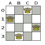
All the constraints have been met, so the solution is correct.
Note that most n queens puzzles have multiple correct solutions. We will focus on finding a single correct solution for a specific n, not on finding the number of possible correct solutions for a specific n.
Problem size
The implementation of the n queens example has not been optimized because it functions as a beginner example. Nevertheless, it can easily handle 64 queens. With a few changes it has been shown to easily handle 5000 queens and more.
3.7.1. Domain model for N queens
This example uses the domain model to solve the four queens problem.
Creating a Domain Model
A good domain model will make it easier to understand and solve your planning problem.
This is the domain model for the n queens example:
Copy to Clipboard Copied! Toggle word wrap Toggle overflow Copy to Clipboard Copied! Toggle word wrap Toggle overflow Copy to Clipboard Copied! Toggle word wrap Toggle overflow Calculating the Search Space.
A
Queeninstance has aColumn(for example: 0 is column A, 1 is column B, …) and aRow(its row, for example: 0 is row 0, 1 is row 1, …).The ascending diagonal line and the descending diagonal line can be calculated based on the column and the row.
The column and row indexes start from the upper left corner of the chessboard.
Copy to Clipboard Copied! Toggle word wrap Toggle overflow Finding the Solution
A single
NQueensinstance contains a list of allQueeninstances. It is theSolutionimplementation which will be supplied to, solved by, and retrieved from the Solver.
Notice that in the four queens example, the NQueens getN() method will always return four.
Figure 3.3. A solution for Four Queens
| columnIndex | rowIndex | ascendingDiagonalIndex (columnIndex + rowIndex) | descendingDiagonalIndex (columnIndex - rowIndex) | |
|---|---|---|---|---|
| A1 | 0 | 1 | 1 (**) | -1 |
| B0 | 1 | 0 (*) | 1 (**) | 1 |
| C2 | 2 | 2 | 4 | 0 |
| D0 | 3 | 0 (*) | 3 | 3 |
When two queens share the same column, row or diagonal line, such as (*) and (**), they can attack each other.
3.8. Cloud balancing
For information about this example, see Red Hat Build of OptaPlanner quick start guides.
3.9. Traveling salesman (TSP - Traveling Salesman Problem)
Given a list of cities, find the shortest tour for a salesman that visits each city exactly once.
The problem is defined by Wikipedia. It is one of the most intensively studied problems in computational mathematics. Yet, in the real world, it is often only part of a planning problem, along with other constraints, such as employee shift rostering constraints.
Problem size
dj38     has  38 cities with a search space of   10^43.
europe40 has  40 cities with a search space of   10^46.
st70     has  70 cities with a search space of   10^98.
pcb442   has 442 cities with a search space of  10^976.
lu980    has 980 cities with a search space of 10^2504.
dj38     has  38 cities with a search space of   10^43.
europe40 has  40 cities with a search space of   10^46.
st70     has  70 cities with a search space of   10^98.
pcb442   has 442 cities with a search space of  10^976.
lu980 has 980 cities with a search space of 10^2504.Problem difficulty
Despite TSP’s simple definition, the problem is surprisingly hard to solve. Because it is an NP-hard problem (like most planning problems), the optimal solution for a specific problem dataset can change a lot when that problem dataset is slightly altered:

3.10. Tennis club scheduling
Every week the tennis club has four teams playing round robin against each other. Assign those four spots to the teams fairly.
Hard constraints:
- Conflict: A team can only play once per day.
- Unavailability: Some teams are unavailable on some dates.
Medium constraints:
- Fair assignment: All teams should play an (almost) equal number of times.
Soft constraints:
- Evenly confrontation: Each team should play against every other team an equal number of times.
Problem size
munich-7teams has 7 teams, 18 days, 12 unavailabilityPenalties and 72 teamAssignments with a search space of 10^60.
munich-7teams has 7 teams, 18 days, 12 unavailabilityPenalties and 72 teamAssignments with a search space of 10^60.Figure 3.4. Domain model

3.11. Meeting scheduling
Assign each meeting to a starting time and a room. Meetings have different durations.
Hard constraints:
- Room conflict: Two meetings must not use the same room at the same time.
- Required attendance: A person cannot have two required meetings at the same time.
- Required room capacity: A meeting must not be in a room that doesn’t fit all of the meeting’s attendees.
- Start and end on same day: A meeting shouldn’t be scheduled over multiple days.
Medium constraints:
- Preferred attendance: A person cannot have two preferred meetings at the same time, nor a preferred and a required meeting at the same time.
Soft constraints:
- Sooner rather than later: Schedule all meetings as soon as possible.
- A break between meetings: Any two meetings should have at least one time grain break between them.
- Overlapping meetings: To minimize the number of meetings in parallel so people don’t have to choose one meeting over the other.
- Assign larger rooms first: If a larger room is available any meeting should be assigned to that room in order to accommodate as many people as possible even if they haven’t signed up to that meeting.
- Room stability: If a person has two consecutive meetings with two or less time grains break between them they better be in the same room.
Problem size
50meetings-160timegrains-5rooms  has  50 meetings, 160 timeGrains and 5 rooms with a search space of 10^145.
100meetings-320timegrains-5rooms has 100 meetings, 320 timeGrains and 5 rooms with a search space of 10^320.
200meetings-640timegrains-5rooms has 200 meetings, 640 timeGrains and 5 rooms with a search space of 10^701.
400meetings-1280timegrains-5rooms has 400 meetings, 1280 timeGrains and 5 rooms with a search space of 10^1522.
800meetings-2560timegrains-5rooms has 800 meetings, 2560 timeGrains and 5 rooms with a search space of 10^3285.
50meetings-160timegrains-5rooms  has  50 meetings, 160 timeGrains and 5 rooms with a search space of 10^145.
100meetings-320timegrains-5rooms has 100 meetings, 320 timeGrains and 5 rooms with a search space of 10^320.
200meetings-640timegrains-5rooms has 200 meetings, 640 timeGrains and 5 rooms with a search space of 10^701.
400meetings-1280timegrains-5rooms has 400 meetings, 1280 timeGrains and 5 rooms with a search space of 10^1522.
800meetings-2560timegrains-5rooms has 800 meetings, 2560 timeGrains and 5 rooms with a search space of 10^3285.3.12. Course timetabling (ITC 2007 Track 3 - Curriculum Course Scheduling)
Schedule each lecture into a timeslot and into a room.
Hard constraints:
- Teacher conflict: A teacher must not have two lectures in the same period.
- Curriculum conflict: A curriculum must not have two lectures in the same period.
- Room occupancy: Two lectures must not be in the same room in the same period.
- Unavailable period (specified per dataset): A specific lecture must not be assigned to a specific period.
Soft constraints:
- Room capacity: A room’s capacity should not be less than the number of students in its lecture.
- Minimum working days: Lectures of the same course should be spread out into a minimum number of days.
- Curriculum compactness: Lectures belonging to the same curriculum should be adjacent to each other (so in consecutive periods).
- Room stability: Lectures of the same course should be assigned to the same room.
The problem is defined by the International Timetabling Competition 2007 track 3.
Problem size
Figure 3.5. Domain model

3.13. Machine reassignment (Google ROADEF 2012)
Assign each process to a machine. All processes already have an original (unoptimized) assignment. Each process requires an amount of each resource (such as CPU or RAM). This is a more complex version of the Cloud Balancing example.
Hard constraints:
- Maximum capacity: The maximum capacity for each resource for each machine must not be exceeded.
- Conflict: Processes of the same service must run on distinct machines.
- Spread: Processes of the same service must be spread out across locations.
- Dependency: The processes of a service depending on another service must run in the neighborhood of a process of the other service.
- Transient usage: Some resources are transient and count towards the maximum capacity of both the original machine as the newly assigned machine.
Soft constraints:
- Load: The safety capacity for each resource for each machine should not be exceeded.
- Balance: Leave room for future assignments by balancing the available resources on each machine.
- Process move cost: A process has a move cost.
- Service move cost: A service has a move cost.
- Machine move cost: Moving a process from machine A to machine B has another A-B specific move cost.
The problem is defined by the Google ROADEF/EURO Challenge 2012.
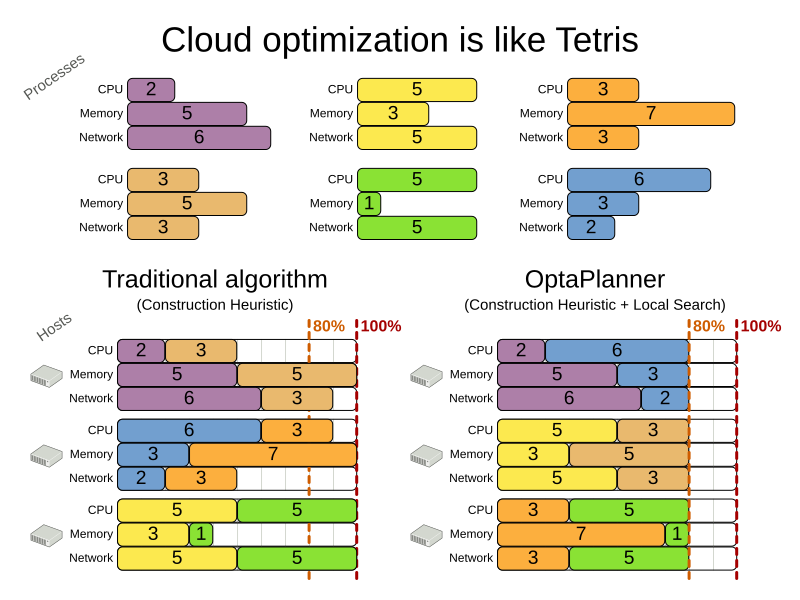
Figure 3.6. Value proposition

Problem size
Figure 3.7. Domain model

3.14. Project job scheduling
Schedule all jobs in time and execution mode to minimize project delays. Each job is part of a project. A job can be executed in different ways: each way is an execution mode that implies a different duration but also different resource usages. This is a form of flexible job shop scheduling.

Hard constraints:
- Job precedence: a job can only start when all its predecessor jobs are finished.
Resource capacity: do not use more resources than available.
- Resources are local (shared between jobs of the same project) or global (shared between all jobs)
- Resources are renewable (capacity available per day) or nonrenewable (capacity available for all days)
Medium constraints:
- Total project delay: minimize the duration (makespan) of each project.
Soft constraints:
- Total makespan: minimize the duration of the whole multi-project schedule.
The problem is defined by the MISTA 2013 challenge.
Problem size
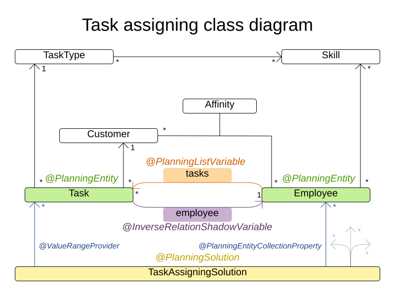
3.15. Task assigning
Assign each task to a spot in an employee’s queue. Each task has a duration which is affected by the employee’s affinity level with the task’s customer.
Hard constraints:
- Skill: Each task requires one or more skills. The employee must possess all these skills.
Soft level 0 constraints:
- Critical tasks: Complete critical tasks first, sooner than major and minor tasks.
Soft level 1 constraints:
Minimize makespan: Reduce the time to complete all tasks.
- Start with the longest working employee first, then the second longest working employee and so forth, to create fairness and load balancing.
Soft level 2 constraints:
- Major tasks: Complete major tasks as soon as possible, sooner than minor tasks.
Soft level 3 constraints:
- Minor tasks: Complete minor tasks as soon as possible.
Figure 3.8. Value proposition

Problem size
24tasks-8employees   has  24 tasks, 6 skills,  8 employees,   4 task types and  4 customers with a search space of   10^30.
50tasks-5employees   has  50 tasks, 5 skills,  5 employees,  10 task types and 10 customers with a search space of   10^69.
100tasks-5employees  has 100 tasks, 5 skills,  5 employees,  20 task types and 15 customers with a search space of  10^164.
500tasks-20employees has 500 tasks, 6 skills, 20 employees, 100 task types and 60 customers with a search space of 10^1168.
24tasks-8employees   has  24 tasks, 6 skills,  8 employees,   4 task types and  4 customers with a search space of   10^30.
50tasks-5employees   has  50 tasks, 5 skills,  5 employees,  10 task types and 10 customers with a search space of   10^69.
100tasks-5employees  has 100 tasks, 5 skills,  5 employees,  20 task types and 15 customers with a search space of  10^164.
500tasks-20employees has 500 tasks, 6 skills, 20 employees, 100 task types and 60 customers with a search space of 10^1168.Figure 3.9. Domain model
3.16. Exam timetabling (ITC 2007 track 1 - Examination)
Schedule each exam into a period and into a room. Multiple exams can share the same room during the same period.

Hard constraints:
- Exam conflict: Two exams that share students must not occur in the same period.
- Room capacity: A room’s seating capacity must suffice at all times.
- Period duration: A period’s duration must suffice for all of its exams.
Period related hard constraints (specified per dataset):
- Coincidence: Two specified exams must use the same period (but possibly another room).
- Exclusion: Two specified exams must not use the same period.
- After: A specified exam must occur in a period after another specified exam’s period.
Room related hard constraints (specified per dataset):
- Exclusive: One specified exam should not have to share its room with any other exam.
Soft constraints (each of which has a parametrized penalty):
- The same student should not have two exams in a row.
- The same student should not have two exams on the same day.
- Period spread: Two exams that share students should be a number of periods apart.
- Mixed durations: Two exams that share a room should not have different durations.
- Front load: Large exams should be scheduled earlier in the schedule.
- Period penalty (specified per dataset): Some periods have a penalty when used.
- Room penalty (specified per dataset): Some rooms have a penalty when used.
It uses large test data sets of real-life universities.
The problem is defined by the International Timetabling Competition 2007 track 1. Geoffrey De Smet finished 4th in that competition with a very early version of OptaPlanner. Many improvements have been made since then.
Problem Size
3.16.1. Domain model for exam timetabling
The following diagram shows the main examination domain classes:
Figure 3.10. Examination domain class diagram

Notice that we’ve split up the exam concept into an Exam class and a Topic class. The Exam instances change during solving (this is the planning entity class), when their period or room property changes. The Topic, Period and Room instances never change during solving (these are problem facts, just like some other classes).
3.17. Nurse rostering (INRC 2010)
For each shift, assign a nurse to work that shift.

Hard constraints:
- No unassigned shifts (built-in): Every shift need to be assigned to an employee.
- Shift conflict: An employee can have only one shift per day.
Soft constraints:
Contract obligations. The business frequently violates these, so they decided to define these as soft constraints instead of hard constraints.
- Minimum and maximum assignments: Each employee needs to work more than x shifts and less than y shifts (depending on their contract).
- Minimum and maximum consecutive working days: Each employee needs to work between x and y days in a row (depending on their contract).
- Minimum and maximum consecutive free days: Each employee needs to be free between x and y days in a row (depending on their contract).
- Minimum and maximum consecutive working weekends: Each employee needs to work between x and y weekends in a row (depending on their contract).
- Complete weekends: Each employee needs to work every day in a weekend or not at all.
- Identical shift types during weekend: Each weekend shift for the same weekend of the same employee must be the same shift type.
- Unwanted patterns: A combination of unwanted shift types in a row, for example a late shift followed by an early shift followed by a late shift.
Employee wishes:
- Day on request: An employee wants to work on a specific day.
- Day off request: An employee does not want to work on a specific day.
- Shift on request: An employee wants to be assigned to a specific shift.
- Shift off request: An employee does not want to be assigned to a specific shift.
- Alternative skill: An employee assigned to a skill should have a proficiency in every skill required by that shift.
The problem is defined by the International Nurse Rostering Competition 2010.
Figure 3.11. Value proposition

Problem size
There are three dataset types:
- Sprint: must be solved in seconds.
- Medium: must be solved in minutes.
- Long: must be solved in hours.
Figure 3.12. Domain model

3.18. Patient admission scheduling
Patient admission scheduling (PAS), also known as hospital bed planning, assigns a bed to each patient that is admitted to the hospital. The bed is assigned to the patient for the duration of the patient’s scheduled stay. Each bed belongs to a room and each room belongs to a department. The arrival and departure dates of the patients are fixed. You only need to assign a bed.
This problem features overconstrained datasets. When it is not necessary to assign all planning entities, it is preferable to assign as many entities as required without breaking hard constraints. This is called overconstrained planning.

Hard constraints:
-
Two patients must not be assigned to the same bed on the same night. Weight:
-1000hard * conflictNightCount. -
A room can have a gender limitation: only females, only males, the same gender in the same night or no gender limitation at all. Weight:
-50hard * nightCount. -
A department can have a minimum or maximum age. Weight:
-100hard * nightCount. -
A patient can require a room with specific equipment. Weight:
-50hard * nightCount.
Medium constraints:
-
Assign every patient to a bed unless the dataset is overconstrained. Weight:
-1medium * nightCount.
Soft constraints:
-
A patient can specify a preference for a maximum room size, for example if the patient wants a single room. Weight:
-8soft * nightCount. -
A patient is best assigned to a department that specializes in the patient’s medical problem. Weight:
-10soft * nightCount. A patient is best assigned to a room that specializes in the patient’s mecical problem. Weight:
-20soft * nightCount.-
The room speciality should be priority 1. Weight:
-10soft * (priority - 1) * nightCount.
-
The room speciality should be priority 1. Weight:
-
A patient can specify a preference for a room with specific equipment. Weight:
-20soft * nightCount.
The problem is a variant on Kaho’s Patient Scheduling and the datasets come from real world hospitals.
Problem size
Figure 3.13. Domain model

3.19. Traveling tournament problem (TTP)
Schedule matches between n number of teams.

Hard constraints:
- Each team plays twice against every other team: once home and once away.
- Each team has exactly one match on each timeslot.
- No team must have more than three consecutive home or three consecutive away matches.
- No repeaters: no two consecutive matches of the same two opposing teams.
Soft constraints:
- Minimize the total distance traveled by all teams.
The problem is defined on Michael Trick’s website (which contains the world records too).
Problem size
3.20. Cheap time scheduling
Schedule all tasks in time and on a machine to minimize power cost. Power prices differ in time. This is a form of job shop scheduling.
Hard constraints:
- Start time limits: Each task must start between its earliest start and latest start limit.
- Maximum capacity: The maximum capacity for each resource for each machine must not be exceeded.
- Startup and shutdown: Each machine must be active in the periods during which it has assigned tasks. Between tasks it is allowed to be idle to avoid startup and shutdown costs.
Medium constraints:
Power cost: Minimize the total power cost of the whole schedule.
- Machine power cost: Each active or idle machine consumes power, which infers a power cost (depending on the power price during that time).
- Task power cost: Each task consumes power too, which infers a power cost (depending on the power price during its time).
- Machine startup and shutdown cost: Every time a machine starts up or shuts down, an extra cost is incurred.
Soft constraints (addendum to the original problem definition):
- Start early: Prefer starting a task sooner rather than later.
The problem is defined by the ICON challenge.
Problem size
3.21. Investment asset class allocation (Portfolio Optimization)
Decide the relative quantity to invest in each asset class.
Hard constraints:
Risk maximum: the total standard deviation must not be higher than the standard deviation maximum.
- Total standard deviation calculation takes asset class correlations into account by applying Markowitz Portfolio Theory.
- Region maximum: Each region has a quantity maximum.
- Sector maximum: Each sector has a quantity maximum.
Soft constraints:
- Maximize expected return.
Problem size
de_smet_1 has 1 regions, 3 sectors and 11 asset classes with a search space of 10^4.
irrinki_1 has 2 regions, 3 sectors and 6 asset classes with a search space of 10^3.
de_smet_1 has 1 regions, 3 sectors and 11 asset classes with a search space of 10^4.
irrinki_1 has 2 regions, 3 sectors and 6 asset classes with a search space of 10^3.Larger datasets have not been created or tested yet, but should not pose a problem. A good source of data is this Asset Correlation website.
3.22. Conference scheduling
Assign each conference talk to a timeslot and a room. Timeslots can overlap. Read and write to and from an *.xlsx file that can be edited with LibreOffice or Excel.
Hard constraints:
- Talk type of timeslot: The type of a talk must match the timeslot’s talk type.
- Room unavailable timeslots: A talk’s room must be available during the talk’s timeslot.
- Room conflict: Two talks can’t use the same room during overlapping timeslots.
- Speaker unavailable timeslots: Every talk’s speaker must be available during the talk’s timeslot.
- Speaker conflict: Two talks can’t share a speaker during overlapping timeslots.
Generic purpose timeslot and room tags:
- Speaker required timeslot tag: If a speaker has a required timeslot tag, then all of his or her talks must be assigned to a timeslot with that tag.
- Speaker prohibited timeslot tag: If a speaker has a prohibited timeslot tag, then all of his or her talks cannot be assigned to a timeslot with that tag.
- Talk required timeslot tag: If a talk has a required timeslot tag, then it must be assigned to a timeslot with that tag.
- Talk prohibited timeslot tag: If a talk has a prohibited timeslot tag, then it cannot be assigned to a timeslot with that tag.
- Speaker required room tag: If a speaker has a required room tag, then all of his or her talks must be assigned to a room with that tag.
- Speaker prohibited room tag: If a speaker has a prohibited room tag, then all of his or her talks cannot be assigned to a room with that tag.
- Talk required room tag: If a talk has a required room tag, then it must be assigned to a room with that tag.
- Talk prohibited room tag: If a talk has a prohibited room tag, then it cannot be assigned to a room with that tag.
- Talk mutually-exclusive-talks tag: Talks that share such a tag must not be scheduled in overlapping timeslots.
- Talk prerequisite talks: A talk must be scheduled after all its prerequisite talks.
Soft constraints:
- Theme track conflict: Minimize the number of talks that share a theme tag during overlapping timeslots.
- Sector conflict: Minimize the number of talks that share a same sector tag during overlapping timeslots.
- Content audience level flow violation: For every content tag, schedule the introductory talks before the advanced talks.
- Audience level diversity: For every timeslot, maximize the number of talks with a different audience level.
- Language diversity: For every timeslot, maximize the number of talks with a different language.
Generic purpose timeslot and room tags:
- Speaker preferred timeslot tag: If a speaker has a preferred timeslot tag, then all of his or her talks should be assigned to a timeslot with that tag.
- Speaker undesired timeslot tag: If a speaker has an undesired timeslot tag, then none of his or her talks should be assigned to a timeslot with that tag.
- Talk preferred timeslot tag: If a talk has a preferred timeslot tag, then it should be assigned to a timeslot with that tag.
- Talk undesired timeslot tag: If a talk has an undesired timeslot tag, then it should not be assigned to a timeslot with that tag.
- Speaker preferred room tag: If a speaker has a preferred room tag, then all of his or her talks should be assigned to a room with that tag.
- Speaker undesired room tag: If a speaker has an undesired room tag, then none of his or her talks should be assigned to a room with that tag.
- Talk preferred room tag: If a talk has a preferred room tag, then it should be assigned to a room with that tag.
- Talk undesired room tag: If a talk has an undesired room tag, then it should not be assigned to a room with that tag.
- Same day talks: All talks that share a theme tag or content tag should be scheduled in the minimum number of days (ideally in the same day).
Figure 3.14. Value proposition

Problem size
18talks-6timeslots-5rooms    has  18 talks,  6 timeslots and  5 rooms with a search space of  10^26.
36talks-12timeslots-5rooms   has  36 talks, 12 timeslots and  5 rooms with a search space of  10^64.
72talks-12timeslots-10rooms  has  72 talks, 12 timeslots and 10 rooms with a search space of 10^149.
108talks-18timeslots-10rooms has 108 talks, 18 timeslots and 10 rooms with a search space of 10^243.
216talks-18timeslots-20rooms has 216 talks, 18 timeslots and 20 rooms with a search space of 10^552.
18talks-6timeslots-5rooms    has  18 talks,  6 timeslots and  5 rooms with a search space of  10^26.
36talks-12timeslots-5rooms   has  36 talks, 12 timeslots and  5 rooms with a search space of  10^64.
72talks-12timeslots-10rooms  has  72 talks, 12 timeslots and 10 rooms with a search space of 10^149.
108talks-18timeslots-10rooms has 108 talks, 18 timeslots and 10 rooms with a search space of 10^243.
216talks-18timeslots-20rooms has 216 talks, 18 timeslots and 20 rooms with a search space of 10^552.3.23. Rock tour
Drive the rock bank bus from show to show, but schedule shows only on available days.
Hard constraints:
- Schedule every required show.
- Schedule as many shows as possible.
Medium constraints:
- Maximize revenue opportunity.
- Minimize driving time.
- Visit sooner than later.
Soft constraints:
- Avoid long driving times.
Problem size
47shows has 47 shows with a search space of 10^59.
47shows has 47 shows with a search space of 10^59.3.24. Flight crew scheduling
Assign flights to pilots and flight attendants.
Hard constraints:
- Required skill: each flight assignment has a required skill. For example, flight AB0001 requires 2 pilots and 3 flight attendants.
- Flight conflict: each employee can only attend one flight at the same time
- Transfer between two flights: between two flights, an employee must be able to transfer from the arrival airport to the departure airport. For example, Ann arrives in Brussels at 10:00 and departs in Amsterdam at 15:00.
- Employee unavailability: the employee must be available on the day of the flight. For example, Ann is on PTO on 1-Feb.
Soft constraints:
- First assignment departing from home
- Last assignment arriving at home
- Load balance flight duration total per employee
Problem size
175flights-7days-Europe  has 2 skills, 50 airports, 150 employees, 175 flights and  875 flight assignments with a search space of  10^1904.
700flights-28days-Europe has 2 skills, 50 airports, 150 employees, 700 flights and 3500 flight assignments with a search space of  10^7616.
875flights-7days-Europe  has 2 skills, 50 airports, 750 employees, 875 flights and 4375 flight assignments with a search space of 10^12578.
175flights-7days-US      has 2 skills, 48 airports, 150 employees, 175 flights and  875 flight assignments with a search space of  10^1904.
175flights-7days-Europe  has 2 skills, 50 airports, 150 employees, 175 flights and  875 flight assignments with a search space of  10^1904.
700flights-28days-Europe has 2 skills, 50 airports, 150 employees, 700 flights and 3500 flight assignments with a search space of  10^7616.
875flights-7days-Europe  has 2 skills, 50 airports, 750 employees, 875 flights and 4375 flight assignments with a search space of 10^12578.
175flights-7days-US has 2 skills, 48 airports, 150 employees, 175 flights and 875 flight assignments with a search space of 10^1904.Chapter 4. Downloading and building Red Hat Build of OptaPlanner examples
You can download the Red Hat Build of OptaPlanner examples as a part of the Red Hat Build of OptaPlanner sources package available on the Red Hat Customer Portal.
Red Hat Build of OptaPlanner has no GUI dependencies. It runs just as well on a server or a mobile JVM as it does on the desktop.
Procedure
Navigate to the Software Downloads page in the Red Hat Customer Portal (login required), and select the product and version from the drop-down options:
- Product: Red Hat Build of OptaPlanner
- Version: 8.38
- Download Red Hat Build of OptaPlanner 8.38 Source Distribution.
Extract the
rhbop-8.38.0-optaplanner-sources.zipfile.The extracted
org.optaplanner.optaplanner-8.38.0.Final-redhat-00004/optaplanner-examples/src/main/java/org/optaplanner/examplesdirectory contains example source code.To build the examples, in the
org.optaplanner.optaplanner-8.38.0.Final-redhat-00004directory enter the following command:mvn clean install -Dquickly
mvn clean install -DquicklyCopy to Clipboard Copied! Toggle word wrap Toggle overflow Change to the examples directory:
optaplanner-examples
optaplanner-examplesCopy to Clipboard Copied! Toggle word wrap Toggle overflow To run the examples, enter the following command:
mvn exec java
mvn exec javaCopy to Clipboard Copied! Toggle word wrap Toggle overflow
Chapter 5. Getting Started with Red Hat Build of OptaPlanner on the Red Hat build of Quarkus platform
Red Hat Build of OptaPlanner is integrated with the Red Hat build of Quarkus platform. Versions of platform artifact dependencies, including OptaPlanner dependencies, are maintained in the Quarkus bill of materials (BOM) file, com.redhat.quarkus.platform:quarkus-bom. You do not need to specify which dependency versions work together. Instead, you can import the Quarkus BOM file to the pom.xml configuration file, where the dependency versions are included in the <dependencyManagement> section. Therefore, you do not need to list the versions of individual Quarkus dependencies that are managed by the specified BOM in the pom.xml file.
Additional resources
- For instructions about using the Maven plug-in to create an OptaPlanner project on the Quarkus platform, see Section 5.2, “Using the Maven plug-in to create an Red Hat Build of OptaPlanner project on the Quarkus platform”.
-
For instructions about using the
code.quarkus.redhat.comwebsite to generate an OptaPlanner project on the Quarkus platform, see Section 5.3, “Using code.quarkus.redhat.com to create an Red Hat Build of OptaPlanner project on the Quarkus platform”. - For instructions about using the CLI to generate an OptaPlanner project on the Quarkus platform, see Section 5.4, “Using the Quarkus CLI to create an Red Hat Build of OptaPlanner project on the Quarkus platform”.
5.1. Apache Maven and Red Hat build of Quarkus
Apache Maven is a distributed build automation tool used in Java application development to create, manage, and build software projects. Maven uses standard configuration files called Project Object Model (POM) files to define projects and manage the build process. POM files describe the module and component dependencies, build order, and targets for the resulting project packaging and output using an XML file. This ensures that the project is built in a correct and uniform manner.
Maven repositories
A Maven repository stores Java libraries, plug-ins, and other build artifacts. The default public repository is the Maven 2 Central Repository, but repositories can be private and internal within a company to share common artifacts among development teams. Repositories are also available from third parties.
You can use the online Maven repository with your Quarkus projects or you can download the Red Hat build of Quarkus Maven repository.
Maven plug-ins
Maven plug-ins are defined parts of a POM file that achieve one or more goals. Quarkus applications use the following Maven plug-ins:
-
Quarkus Maven plug-in (
quarkus-maven-plugin): Enables Maven to create Quarkus projects, supports the generation of uber-JAR files, and provides a development mode. -
Maven Surefire plug-in (
maven-surefire-plugin): Used during the test phase of the build lifecycle to execute unit tests on your application. The plug-in generates text and XML files that contain the test reports.
5.1.1. Configuring the Maven settings.xml file for the online repository
You can use the online Maven repository with your Maven project by configuring your user settings.xml file. This is the recommended approach. Maven settings used with a repository manager or repository on a shared server provide better control and manageability of projects.
When you configure the repository by modifying the Maven settings.xml file, the changes apply to all of your Maven projects.
Procedure
Open the Maven
~/.m2/settings.xmlfile in a text editor or integrated development environment (IDE).NoteIf there is not a
settings.xmlfile in the~/.m2/directory, copy thesettings.xmlfile from the$MAVEN_HOME/.m2/conf/directory into the~/.m2/directory.Add the following lines to the
<profiles>element of thesettings.xmlfile:Copy to Clipboard Copied! Toggle word wrap Toggle overflow Add the following lines to the
<activeProfiles>element of thesettings.xmlfile and save the file.<activeProfile>red-hat-enterprise-maven-repository</activeProfile>
<activeProfile>red-hat-enterprise-maven-repository</activeProfile>Copy to Clipboard Copied! Toggle word wrap Toggle overflow
5.1.2. Downloading and configuring the Quarkus Maven repository
If you do not want to use the online Maven repository, you can download and configure the Quarkus Maven repository to create a Quarkus application with Maven. The Quarkus Maven repository contains many of the requirements that Java developers typically use to build their applications. This procedure describes how to edit the settings.xml file to configure the Quarkus Maven repository.
When you configure the repository by modifying the Maven settings.xml file, the changes apply to all of your Maven projects.
Procedure
- Download the Red Hat build of Quarkus Maven repository ZIP file from the Software Downloads page of the Red Hat Customer Portal (login required).
- Expand the downloaded archive.
-
Change directory to the
~/.m2/directory and open the Mavensettings.xmlfile in a text editor or integrated development environment (IDE). Add the following lines to the
<profiles>element of thesettings.xmlfile, whereQUARKUS_MAVEN_REPOSITORYis the path of the Quarkus Maven repository that you downloaded. The format ofQUARKUS_MAVEN_REPOSITORYmust befile://$PATH, for examplefile:///home/userX/rh-quarkus-2.13.8.GA-maven-repository/maven-repository.Copy to Clipboard Copied! Toggle word wrap Toggle overflow Add the following lines to the
<activeProfiles>element of thesettings.xmlfile and save the file.<activeProfile>red-hat-quarkus-maven-repository</activeProfile>
<activeProfile>red-hat-quarkus-maven-repository</activeProfile>Copy to Clipboard Copied! Toggle word wrap Toggle overflow
If your Maven repository contains outdated artifacts, you might encounter one of the following Maven error messages when you build or deploy your project, where ARTIFACT_NAME is the name of a missing artifact and PROJECT_NAME is the name of the project you are trying to build:
-
Missing artifact PROJECT_NAME -
[ERROR] Failed to execute goal on project ARTIFACT_NAME; Could not resolve dependencies for PROJECT_NAME
To resolve the issue, delete the cached version of your local repository located in the ~/.m2/repository directory to force a download of the latest Maven artifacts.
5.2. Using the Maven plug-in to create an Red Hat Build of OptaPlanner project on the Quarkus platform
You can get up and running with an Red Hat Build of OptaPlanner and Quarkus application using Apache Maven and the Quarkus Maven plug-in.
Prerequisites
- OpenJDK 11 or later is installed. Red Hat build of Open JDK is available from the Software Downloads page in the Red Hat Customer Portal (login required).
- Apache Maven 3.8 or higher is installed. Maven is available from the Apache Maven Project website.
Procedure
In a command terminal, enter the following command to verify that Maven is using JDK 11 and that the Maven version is 3.8 or higher:
mvn --version
mvn --versionCopy to Clipboard Copied! Toggle word wrap Toggle overflow - If the preceding command does not return JDK 11, add the path to JDK 11 to the PATH environment variable and enter the preceding command again.
To generate a Quarkus OptaPlanner quickstart project, enter the following command, where
redhat-0000xis the current version of the Quarkus BOM file:Copy to Clipboard Copied! Toggle word wrap Toggle overflow This command create the following elements in the
./optaplanner-quickstartdirectory:- The Maven structure
-
Example
Dockerfilefile insrc/main/docker The application configuration file
Expand Table 5.1. Properties used in the mvn io.quarkus:quarkus-maven-plugin:2.13.8.SP1-redhat-0000x:create command Property Description projectGroupIdThe group ID of the project.
projectArtifactIdThe artifact ID of the project.
extensionsA comma-separated list of Quarkus extensions to use with this project. For a full list of Quarkus extensions, enter
mvn quarkus:list-extensionson the command line.noExamplesCreates a project with the project structure but without tests or classes.
The values of the
projectGroupIDand theprojectArtifactIDproperties are used to generate the project version. The default project version is1.0.0-SNAPSHOT.
To view your OptaPlanner project, change directory to the OptaPlanner Quickstarts directory:
cd optaplanner-quickstart
cd optaplanner-quickstartCopy to Clipboard Copied! Toggle word wrap Toggle overflow Review the
pom.xmlfile. The content should be similar to the following example:Copy to Clipboard Copied! Toggle word wrap Toggle overflow
5.3. Using code.quarkus.redhat.com to create an Red Hat Build of OptaPlanner project on the Quarkus platform
You can use the code.quarkus.redhat.com website to generate an Red Hat Build of OptaPlanner Quarkus Maven project and automatically add and configure the extensions that you want to use in your application.
This section walks you through the process of generating an OptaPlanner Maven project and includes the following topics:
- Specifying basic details about your application.
- Choosing the extensions that you want to include in your project.
- Generating a downloadable archive with your project files.
- Using the custom commands for compiling and starting your application.
Prerequisites
- You have a web browser.
Procedure
-
Open
https://code.quarkus.redhat.comin your web browser: - Specify details about your project:
-
Enter a group name for your project. The format of the name follows the Java package naming convention, for example,
com.example. -
Enter a name that you want to use for Maven artifacts generated from your project, for example
code-with-quarkus. Select Build Tool > Maven to specify that you want to create a Maven project. The build tool that you choose determines the items:
- The directory structure of your generated project
- The format of configuration files used in your generated project
The custom build script and command for compiling and starting your application that
code.quarkus.redhat.comdisplays for you after you generate your projectNoteRed Hat provides support for using
code.quarkus.redhat.comto create OptaPlanner Maven projects only. Generating Gradle projects is not supported by Red Hat.
-
Enter a version to be used in artifacts generated from your project. The default value of this field is
1.0.0-SNAPSHOT. Using semantic versioning is recommended, but you can use a different type of versioning if you prefer. Enter the package name of artifacts that the build tool generates when you package your project.
According to the Java package naming conventions the package name should match the group name that you use for your project, but you can specify a different name.
Select the following extensions to include as dependencies:
- RESTEasy JAX-RS (quarkus-resteasy)
- RESTEasy Jackson (quarkus-resteasy-jackson)
- OptaPlanner AI constraint solver(optaplanner-quarkus)
OptaPlanner Jackson (optaplanner-quarkus-jackson)
Red Hat provides different levels of support for individual extensions on the list, which are indicated by labels next to the name of each extension:
- SUPPORTED extensions are fully supported by Red Hat for use in enterprise applications in production environments.
- TECH-PREVIEW extensions are subject to limited support by Red Hat in production environments under the Technology Preview Features Support Scope.
- DEV-SUPPORT extensions are not supported by Red Hat for use in production environments, but the core functionalities that they provide are supported by Red Hat developers for use in developing new applications.
DEPRECATED extension are planned to be replaced with a newer technology or implementation that provides the same functionality.
Unlabeled extensions are not supported by Red Hat for use in production environments.
- Select Generate your application to confirm your choices and display the overlay screen with the download link for the archive that contains your generated project. The overlay screen also shows the custom command that you can use to compile and start your application.
- Select Download the ZIP to save the archive with the generated project files to your system.
- Extract the contents of the archive.
Navigate to the directory that contains your extracted project files:
cd <directory_name>
cd <directory_name>Copy to Clipboard Copied! Toggle word wrap Toggle overflow Compile and start your application in development mode:
./mvnw compile quarkus:dev
./mvnw compile quarkus:devCopy to Clipboard Copied! Toggle word wrap Toggle overflow
5.4. Using the Quarkus CLI to create an Red Hat Build of OptaPlanner project on the Quarkus platform
You can use the Quarkus command line interface (CLI) to create a Quarkus OptaPlanner project.
Prerequisites
- You have installed the Quarkus CLI. For information, see Building Quarkus Apps with Quarkus Command Line Interface.
Procedure
Create a Quarkus application:
quarkus create app -P io.quarkus:quarkus-bom:2.13.8.SP1-redhat-0000x
quarkus create app -P io.quarkus:quarkus-bom:2.13.8.SP1-redhat-0000xCopy to Clipboard Copied! Toggle word wrap Toggle overflow To view the available extensions, enter the following command:
quarkus ext -i
quarkus ext -iCopy to Clipboard Copied! Toggle word wrap Toggle overflow This command returns the following extensions:
optaplanner-quarkus
optaplanner-quarkus-benchmark
optaplanner-quarkus-jackson
optaplanner-quarkus-jsonb
optaplanner-quarkus
optaplanner-quarkus-benchmark
optaplanner-quarkus-jackson
optaplanner-quarkus-jsonb
Copy to Clipboard Copied! Toggle word wrap Toggle overflow Enter the following command to add extensions to the project’s
pom.xmlfile:quarkus ext add resteasy-jackson quarkus ext add optaplanner-quarkus quarkus ext add optaplanner-quarkus-jackson
quarkus ext add resteasy-jackson quarkus ext add optaplanner-quarkus quarkus ext add optaplanner-quarkus-jacksonCopy to Clipboard Copied! Toggle word wrap Toggle overflow Open the
pom.xmlfile in a text editor. The contents of the file should look similar to the following example:Copy to Clipboard Copied! Toggle word wrap Toggle overflow
Part III. The Red Hat Build of OptaPlanner solver
Solving a planning problem with OptaPlanner consists of the following steps:
-
Model your planning problem as a class annotated with the
@PlanningSolutionannotation (for example, theNQueensclass). -
Configure a Solver (for example a First Fit and Tabu Search solver for any
NQueensinstance). - Load a problem data set from your data layer (for example a Four Queens instance). That is the planning problem.
-
Solve it with
Solver.solve(problem), which returns the best solution found.

Chapter 6. Configuring the Red Hat Build of OptaPlanner solver
You can use the following methods to configure your OptaPlanner solver:
- Use an XML file.
-
Use the
SolverConfigAPI. - Add class annotations and JavaBean property annotations on the domain model.
- Control the method that OptaPlanner uses to access your domain.
- Define custom properties.
6.1. Using an XML file to configure the OptaPlanner solver
Each example project has a solver configuration file that you can edit. The <EXAMPLE>SolverConfig.xml file is located in the org.optaplanner.optaplanner-8.38.0.Final-redhat-00004/optaplanner-examples/src/main/resources/org/optaplanner/examples/<EXAMPLE> directory, where <EXAMPLE> is the name of the OptaPlanner example project. Alternatively, you can create a SolverFactory from a file with SolverFactory.createFromXmlFile(). However, for portability reasons, a classpath resource is recommended.
Both a Solver and a SolverFactory have a generic type called Solution_, which is the class representing a planning problem and solution.
OptaPlanner makes it relatively easy to switch optimization algorithms by changing the configuration.
Procedure
-
Build a
Solverinstance with theSolverFactory. Configure the solver configuration XML file:
- Define the model.
- Define the score function.
Optional: Configure the optimization algorithm.
The following example is a solver XML file for the NQueens problem:
Copy to Clipboard Copied! Toggle word wrap Toggle overflow NoteOn some environments, for example OSGi and JBoss modules, classpath resources such as the solver config, score DRLs, and domain classe) in your JAR files might not be available to the default
ClassLoaderof theoptaplanner-coreJAR file. In those cases, provide theClassLoaderof your classes as a parameter:SolverFactory<NQueens> solverFactory = SolverFactory.createFromXmlResource( ".../nqueensSolverConfig.xml", getClass().getClassLoader());SolverFactory<NQueens> solverFactory = SolverFactory.createFromXmlResource( ".../nqueensSolverConfig.xml", getClass().getClassLoader());Copy to Clipboard Copied! Toggle word wrap Toggle overflow
Configure the
SolverFactorywith a solver configuration XML file, provided as a classpath resource as defined byClassLoader.getResource():SolverFasctory<NQueens> solverFactory = SolverFactory.createFromXmlResource( "org/optaplanner/examples/nqueens/optional/nqueensSolverConfig.xml"); Solver<NQueens> solver = solverFactory.buildSolver();SolverFasctory<NQueens> solverFactory = SolverFactory.createFromXmlResource( "org/optaplanner/examples/nqueens/optional/nqueensSolverConfig.xml"); Solver<NQueens> solver = solverFactory.buildSolver();Copy to Clipboard Copied! Toggle word wrap Toggle overflow
6.2. Using the Java API to configure the OptaPlanner solver
You can configure a solver by using the SolverConfig API. This is especially useful to change values dynamically at runtime. The following example changes the running time based on system properties before building the Solver in the NQueens project:
Every element in the solver configuration XML file is available as a Config class or a property on a Config class in the package namespace org.optaplanner.core.config. These Config classes are the Java representation of the XML format. They build the runtime components of the package namespace org.optaplanner.core.impl and assemble them into an efficient Solver.
To configure a SolverFactory dynamically for each user request, build a template SolverConfig during initialization and copy it with the copy constructor for each user request. The following example shows how to do this with the NQueens problem:
6.3. OptaPlanner annotation
You must specify which classes in your domain model are planning entities, which properties are planning variables, and so on. Use one of the following methods to add annotations to your OptaPlanner project:
- Add class annotations and JavaBean property annotations on the domain model. The property annotations must be on the getter method, not on the setter method. Annotated getter methods do not need to be public. This is the recommended method.
- Add class annotations and field annotations on the domain model. Annotated fields do not need to be public.
6.4. Specifying OptaPlanner domain access
By default, OptaPlanner accesses your domain using reflection. Reflection is reliable but slow compared to direct access. Alternatively, you can configure OptaPlanner to access your domain using Gizmo, which will generate bytecode that directly accesses the fields and methods of your domain without reflection. However, this method has the following restrictions:
- The planning annotations can only be on public fields and public getters.
-
io.quarkus.gizmo:gizmomust be on the classpath.
These restrictions do not apply when you use OptaPlanner with Quarkus because Gizmo is the default domain access type.
Procedure
To use Gizmo outside of Quarkus, set the domainAccessType in the solver configuration:
  <solver>
    <domainAccessType>GIZMO</domainAccessType>
  </solver>
  <solver>
    <domainAccessType>GIZMO</domainAccessType>
</solver>6.5. Configuring custom properties
In your OptaPlanner projects, you can add custom properties to solver configuration elements that instantiate classes and have documents that explicitly mention custom properties.
Prerequisites
- You have a solver.
Procedure
Add a custom property.
For example, if your
EasyScoreCalculatorhas heavy calculations which are cached and you want to increase the cache size in one benchmark add themyCacheSizeproperty:Copy to Clipboard Copied! Toggle word wrap Toggle overflow Add a public setter for each custom property, which is called when a
Solveris built.Copy to Clipboard Copied! Toggle word wrap Toggle overflow Most value types are supported, including
boolean,int,double,BigDecimal,Stringandenums.
Chapter 7. Using the OptaPlanner solver
A solver finds the best and optimal solution to your planning problem. A solver can only solve one planning problem instance at a time. Solvers are built with the SolverFactory method:
A solver should only be accessed from a single thread, except for the methods that are specifically documented in javadoc as being thread-safe. The solve() method hogs the current thread. Hogging the thread can cause HTTP timeouts for REST services and it requires extra code to solve multiple data sets in parallel. To avoid such issues, use a SolverManager instead.
7.1. Solving a problem
Use the solver to solve a planning problem.
Prerequisites
-
A
Solverbuilt from a solver configuration -
An
@PlanningSolutionannotation that represents the planning problem instance
Procedure
Provide the planning problem as an argument to the solve() method. The solver will return the best solution found.
The following example solves the NQueens problem:
    NQueens problem = ...;
    NQueens bestSolution = solver.solve(problem);
    NQueens problem = ...;
    NQueens bestSolution = solver.solve(problem);
In this example, the solve() method will return an NQueens instance with every Queen assigned to a Row.
The solution instance given to the solve(Solution) method can be partially or fully initialized, which is often the case in repeated planning.
Figure 7.1. Best Solution for the Four Queens Puzzle in 8ms (Also an Optimal Solution)
The solve(Solution) method can take a long time depending on the problem size and the solver configuration. The Solver intelligently works through the search space of possible solutions and remembers the best solution it encounters during solving. Depending on a number of factors, including problem size, how much time the Solver has, the solver configuration, and so forth, the best solution might or might not be an optimal solution.
The solution instance given to the method solve(Solution) is changed by the Solver, but do not mistake it for the best solution.
The solution instance returned by the methods solve(Solution) or getBestSolution() is most likely a planning clone of the instance given to the method solve(Solution), which implies it is a different instance.
7.2. Solver environment mode
The solver environment mode enables you to detect common bugs in your implementation. It does not affect the logging level.
A solver has a single random instance. Some solver configurations use the random instance a lot more than others. For example, the Simulated Annealing algorithm depends highly on random numbers, while Tabu Search only depends on it to resolve score ties. The environment mode influences the seed of that random instance.
You can set the environment mode in the solver configuration XML file. The following example sets the FAST_ASSERT mode:
<solver xmlns="https://www.optaplanner.org/xsd/solver" xmlns:xsi="http://www.w3.org/2001/XMLSchema-instance"
    xsi:schemaLocation="https://www.optaplanner.org/xsd/solver https://www.optaplanner.org/xsd/solver/solver.xsd">
  <environmentMode>FAST_ASSERT</environmentMode>
  ...
</solver>
<solver xmlns="https://www.optaplanner.org/xsd/solver" xmlns:xsi="http://www.w3.org/2001/XMLSchema-instance"
    xsi:schemaLocation="https://www.optaplanner.org/xsd/solver https://www.optaplanner.org/xsd/solver/solver.xsd">
  <environmentMode>FAST_ASSERT</environmentMode>
  ...
</solver>The following list describes the environment modes that you can use in the solver configuration file:
-
FULL_ASSERTmode turns on all assertions, for example the assertion that the incremental score calculation is uncorrupted for each move, to fail-fast on a bug in a Move implementation, a constraint, the engine itself, and so on. This mode is reproducible. It is also intrusive because it calls the methodcalculateScore()more frequently than a non-assert mode. TheFULL_ASSERTmode is very slow because it does not rely on incremental score calculation.
-
NON_INTRUSIVE_FULL_ASSERTmode turns on several assertions to fail-fast on a bug in a Move implementation, a constraint, the engine itself, and so on. This mode is reproducible. It is non-intrusive because it does not call the methodcalculateScore()more frequently than a non assert mode. TheNON_INTRUSIVE_FULL_ASSERTmode is very slow because it does not rely on incremental score calculation.
-
FAST_ASSERTmode turns on most assertions, such as the assertions that an undoMove’s score is the same as before the Move, to fail-fast on a bug in a Move implementation, a constraint, the engine itself, and so on. This mode is reproducible. It is also intrusive because it calls the methodcalculateScore()more frequently than a non-assert mode. TheFAST_ASSERTmode is slow. Write a test case that does a short run of your planning problem with theFAST_ASSERTmode on.
REPRODUCIBLEmode is the default mode because it is recommended during development. In this mode, two runs in the same OptaPlanner version execute the same code in the same order. Those two runs have the same result at every step, except if the following note applies. This enables you to reproduce bugs consistently. It also enables you to benchmark certain refactorings, such as a score constraint performance optimization, fairly across runs.NoteDespite using
REPRODCIBLEmode, your application might still not be fully reproducible for the following reasons:-
Use of
HashSetor anotherCollectionwhich has an inconsistent order between JVM runs for collections of planning entities or planning values but not normal problem facts, especially in the solution implementation. Replace it withLinkedHashSet. - Combining a time gradient dependent algorithm, most notably the Simulated Annealing algorithm, together with time spent termination. A sufficiently large difference in allocated CPU time will influence the time gradient values. Replace the Simulated Annealing algorithms with the Late Acceptance algorithm, or replace time spent termination with step count termination.
-
Use of
-
REPRODUCIBLEmode can be slightly slower thanNON_REPRODUCIBLEmode. If your production environment can benefit from reproducibility, use this mode in production. In practice,REPRODUCIBLEmode uses the default fixed random seed if no seed is specified and it also disables certain concurrency optimizations such as work stealing.
-
NON_REPRODUCIBLEmode can be slightly faster thanREPRODUCIBLEmode. Avoid using it during development because it makes debugging and bug fixing difficult. If reproducibility isn’t important in your production environment, useNON_REPRODUCIBLEmode in production. In practice, this mode uses no fixed random seed if no seed is specified.
7.3. Changing the OptaPlanner solver logging level
You can change the logging level in an OptaPlanner solver to review solver activity. The following list describes the different logging levels:
error: Logs errors, except those that are thrown to the calling code as a
RuntimeException.If an error occurs, OptaPlanner normally fails fast. It throws a subclass of
RuntimeExceptionwith a detailed message to the calling code. To avoid duplicate log messages, it does not log it as an error. Unless the calling code explicitly catches and eliminates thatRuntimeException, aThread’s default `ExceptionHandlerwill log it as an error anyway. Meanwhile, the code is disrupted from doing further harm or obfuscating the error.- warn: Logs suspicious circumstances
- info: Logs every phase and the solver itself
- debug: Logs every step of every phase
- trace: Logs every move of every step of every phase
Specifying trace logging will slow down performance considerably. However, trace logging is invaluable during development to discover a bottleneck.
Even debug logging can slow down performance considerably for fast stepping algorithms such as Late Acceptance and Simulated Annealing, but not for slow stepping algorithms such as Tabu Search.
Both trace` and debug logging cause congestion in multithreaded solving with most appenders.
In Eclipse, debug logging to the console tends to cause congestion with score calculation speeds above 10000 per second. Neither IntelliJ or the Maven command line suffer from this problem.
Procedure
Set the logging level to debug logging to see when the phases end and how fast steps are taken.
The following example shows output from debug logging:
All time spent values are in milliseconds.
Everything is logged to SLF4J, which is a simple logging facade that delegates every log message to Logback, Apache Commons Logging, Log4j, or java.util.logging. Add a dependency to the logging adaptor for your logging framework of choice.
7.4. Using Logback to log OptaPlanner solver activity
Logback is the recommended logging frameworkd to use with OptaPlanner. Use Logback to log OptaPlanner solver activity.
Prerequisites
- You have an OptaPlanner project.
Procedure
Add the following Maven dependency to your OptaPlanner project’s
pom.xmlfile:NoteYou do not need to add an extra bridge dependency.
    <dependency>
      <groupId>ch.qos.logback</groupId>
      <artifactId>logback-classic</artifactId>
      <version>1.x</version>
    </dependency>
<dependency> <groupId>ch.qos.logback</groupId> <artifactId>logback-classic</artifactId> <version>1.x</version> </dependency>Copy to Clipboard Copied! Toggle word wrap Toggle overflow Configure the logging level on the
org.optaplannerpackage in yourlogback.xmlfile as shown in the following example where<LEVEL>is a logging level listed in Section 7.4, “Using Logback to log OptaPlanner solver activity”.Copy to Clipboard Copied! Toggle word wrap Toggle overflow Optional: If you have a multitenant application where multiple
Solverinstances might be running at the same time, separate the logging of each instance into separate files:Surround the
solve()call with Mapped Diagnostic Context (MDC):MDC.put("tenant.name",tenantName); MySolution bestSolution = solver.solve(problem); MDC.remove("tenant.name");MDC.put("tenant.name",tenantName); MySolution bestSolution = solver.solve(problem); MDC.remove("tenant.name");Copy to Clipboard Copied! Toggle word wrap Toggle overflow Configure your logger to use different files for each
${tenant.name}. For example, use aSiftingAppenderin thelogback.xmlfile:Copy to Clipboard Copied! Toggle word wrap Toggle overflow NoteWhen running multiple solvers or one multithreaded solve, most appenders, including the console, cause congestion with
debugandtracelogging. Switch to an async appender to avoid this problem or turn offdebuglogging.
-
If OptaPlanner doesn’t recognize the new level, temporarily add the system property
-Dlogback.LEVEL=trueto troubleshoot.
7.5. Using Log4J to log OptaPlanner solver activity
If you are already using Log4J and you do not want to switch to its faster successor, Logback, you can configure your OptaPlanner project for Log4J.
Prerequisites
- You have an OptaPlanner project
- You are using the Log4J logging framework
Procedure
Add the bridge dependency to the project
pom.xmlfile:<dependency> <groupId>org.slf4j</groupId> <artifactId>slf4j-log4j12</artifactId> <version>1.x</version> </dependency><dependency> <groupId>org.slf4j</groupId> <artifactId>slf4j-log4j12</artifactId> <version>1.x</version> </dependency>Copy to Clipboard Copied! Toggle word wrap Toggle overflow Configure the logging level on the package
org.optaplannerin yourlog4j.xmlfile as shown in the following example, where<LEVEL>is a logging level listed in Section 7.4, “Using Logback to log OptaPlanner solver activity”.Copy to Clipboard Copied! Toggle word wrap Toggle overflow Optional: If you have a multitenant application where multiple
Solverinstances might be running at the same time, separate the logging of each instance into separate files:Surround the
solve()call with Mapped Diagnostic Context (MDC):MDC.put("tenant.name",tenantName); MySolution bestSolution = solver.solve(problem); MDC.remove("tenant.name");MDC.put("tenant.name",tenantName); MySolution bestSolution = solver.solve(problem); MDC.remove("tenant.name");Copy to Clipboard Copied! Toggle word wrap Toggle overflow Configure your logger to use different files for each
${tenant.name}. For example, use aSiftingAppenderin thelogback.xmlfile:Copy to Clipboard Copied! Toggle word wrap Toggle overflow NoteWhen running multiple solvers or one multithreaded solve, most appenders, including the console, cause congestion with
debugandtracelogging. Switch to an async appender to avoid this problem or turn offdebuglogging.
7.6. Monitoring the solver
OptaPlanner exposes metrics through Micrometer, a metrics instrumentation library for Java applications. You can use Micrometer with popular monitoring systems to monitor the OptaPlanner solver.
7.6.1. Configuring a Quarkus OptaPlanner application for Micrometer
To configure your OptaPlanner Quarkus application to use Micrometer and a specified monitoring system, add the Micrometer dependency to the pom.xml file.
Prerequisites
- You have a Quarkus OptaPlanner application.
Procedure
Add the following dependency to your application’s
pom.xmlfile where<MONITORING_SYSTEM>is a monitoring system supported by Micrometer and Quarkus:NotePrometheus is currently the only monitoring system supported by Quarkus.
<dependency>
 <groupId>io.quarkus</groupId>
 <artifactId>quarkus-micrometer-registry-<MONITORING_SYSTEM></artifactId>
</dependency>
<dependency>
 <groupId>io.quarkus</groupId>
 <artifactId>quarkus-micrometer-registry-<MONITORING_SYSTEM></artifactId>
</dependency>
Copy to Clipboard Copied! Toggle word wrap Toggle overflow To run the application in development mode, enter the following command:
mvn compile quarkus:dev
mvn compile quarkus:devCopy to Clipboard Copied! Toggle word wrap Toggle overflow To view metrics for your application, enter the following URL in a browser:
http://localhost:8080/q/metrics
http://localhost:8080/q/metricsCopy to Clipboard Copied! Toggle word wrap Toggle overflow
7.6.2. Configuring a Spring Boot OptaPlanner application for Micrometer
To configure your Spring Boot OptaPlanner application to use Micrometer and a specified monitoring system, add the Micrometer dependency to the pom.xml file.
Prerequisites
- You have a Spring Boot OptaPlanner application.
Procedure
Add the following dependency to your application’s
pom.xmlfile where<MONITORING_SYSTEM>is a monitoring system supported by Micrometer and Spring Boot:Copy to Clipboard Copied! Toggle word wrap Toggle overflow -
Add configuration information to the application’s
application.propertiesfile. For information, see the Micrometer web site. To run the application, enter the following command:
mvn spring-boot:run
mvn spring-boot:runCopy to Clipboard Copied! Toggle word wrap Toggle overflow To view metrics for your application, enter the following URL in a browser:
http://localhost:8080/actuator/metrics
NoteUse the following URL as the Prometheus scraper path:
http://localhost:8080/actuator/prometheus
7.6.3. Configuring a plain Java OptaPlanner application for Micrometer
To configuring a plain Java OptaPlanner application to use Micrometer, you must add Micrometer dependencies and configuration information for your chosen monitoring system to your project’s POM.XML file.
Prerequisites
- You have a plain Java OptaPlanner application.
Procedure
Add the following dependencies to your application’s
pom.xmlfile where<MONITORING_SYSTEM>is a monitoring system that is configured with Micrometer and<VERSION>is the version of Micrometer that you are using:Copy to Clipboard Copied! Toggle word wrap Toggle overflow -
Add Micrometer configuration information for your monitoring system to the beginning of your project’s
pom.xmlfile. For information, see the Micrometer web site. Add the following line below the configuration information, where
<MONITORING_SYSTEM>is the monitoring system that you added:Metrics.addRegistry(<MONITORING_SYSTEM>);
Metrics.addRegistry(<MONITORING_SYSTEM>);Copy to Clipboard Copied! Toggle word wrap Toggle overflow The following example shows how to add the Prometheus monitoring system:
Copy to Clipboard Copied! Toggle word wrap Toggle overflow Open your monitoring system to view the metrics for your OptaPlanner project. The following metrics are exposed:
NoteThe names and format of the metrics vary depending on the registry.
-
optaplanner.solver.errors.total: the total number of errors that occurred while solving since the start of the measuring. -
optaplanner.solver.solve-length.active-count: the number of solvers currently solving. -
optaplanner.solver.solve-length.seconds-max: run time of the longest-running currently active solver. -
optaplanner.solver.solve-length.seconds-duration-sum: the sum of each active solver’s solve duration. For example, if there are two active solvers, one running for three minutes and the other for one minute, the total solve time is four minutes.
-
7.6.4. Additional Metrics
For more detailed monitoring, you can configure OptaPlanner in the solver configuration to monitor additional metrics at a performance cost. The following example uses the BEST_SCORE and SCORE_CALCULATION_COUNT metric :
You can enable the following metrics in this configuration:
-
SOLVE_DURATION(enabled by default, Micrometer meter ID:optaplanner.solver.solve.duration): Measures the duration of solving for the longest active solver, the number of active solvers, and the cumulative duration of all active solvers. -
ERROR_COUNT(enabled by default, Micrometer meter ID:optaplanner.solver.errors): Measures the number of errors that occurred while solving. -
SCORE_CALCULATION_COUNT(enabled by default, Micrometer meter ID:optaplanner.solver.score.calculation.count): Measures the number of score calculations the OptaPlanner performed. -
BEST_SCORE(Micrometer meter ID:optaplanner.solver.best.score.*): Measures the score of the best solution that OptaPlanner has found so far. There are separate meters for each level of the score. For instance, for aHardSoftScore, there areoptaplanner.solver.best.score.hard.scoreandoptaplanner.solver.best.score.soft.scoremeters. -
STEP_SCORE(Micrometer meter ID:optaplanner.solver.step.score.*): Measures the score of each step that OptaPlanner takes. There are separate meters for each level of the score. For instance, for aHardSoftScore, there areoptaplanner.solver.step.score.hard.scoreandoptaplanner.solver.step.score.soft.scoremeters. -
BEST_SOLUTION_MUTATION(Micrometer meter ID:optaplanner.solver.best.solution.mutation): Measures the number of changed planning variables between consecutive best solutions. -
MOVE_COUNT_PER_STEP(Micrometer meter ID:optaplanner.solver.step.move.count): Measures the number of moves evaluated in a step. -
MEMORY_USE(Micrometer meter ID:jvm.memory.used): Measures the amount of memory used across the JVM. This metric does not measure the amount of memory used by a solver; two solvers on the same JVM will report the same value for this metric. -
CONSTRAINT_MATCH_TOTAL_BEST_SCORE(Micrometer meter ID:optaplanner.solver.constraint.match.best.score.*): Measures the score impact of each constraint on the best solution that OptaPlanner has found so far. There are separate meters for each level of the score, with tags for each constraint. For instance, for aHardSoftScorefor a constraint "Minimize Cost" in package "com.example", there areoptaplanner.solver.constraint.match.best.score.hard.scoreandoptaplanner.solver.constraint.match.best.score.soft.scoremeters with tags "constraint.package=com.example" and "constraint.name=Minimize Cost". -
CONSTRAINT_MATCH_TOTAL_STEP_SCORE(Micrometer meter ID:optaplanner.solver.constraint.match.step.score.*): Measures the score impact of each constraint on the current step. There are separate meters for each level of the score, with tags for each constraint. For instance, for aHardSoftScorefor a constraint "Minimize Cost" in package "com.example", there areoptaplanner.solver.constraint.match.step.score.hard.scoreandoptaplanner.solver.constraint.match.step.score.soft.scoremeters with tags "constraint.package=com.example" and "constraint.name=Minimize Cost". -
PICKED_MOVE_TYPE_BEST_SCORE_DIFF(Micrometer meter ID:optaplanner.solver.move.type.best.score.diff.*): Measures how much a particular move type improves the best solution. There are separate meters for each level of the score, with a tag for the move type. For instance, for aHardSoftScoreand aChangeMovefor the computer of a process, there areoptaplanner.solver.move.type.best.score.diff.hard.scoreandoptaplanner.solver.move.type.best.score.diff.soft.scoremeters with the tagmove.type=ChangeMove(Process.computer). -
PICKED_MOVE_TYPE_STEP_SCORE_DIFF(Micrometer meter ID:optaplanner.solver.move.type.step.score.diff.*): Measures how much a particular move type improves the best solution. There are separate meters for each level of the score, with a tag for the move type. For instance, for aHardSoftScoreand aChangeMovefor the computer of a process, there areoptaplanner.solver.move.type.step.score.diff.hard.scoreandoptaplanner.solver.move.type.step.score.diff.soft.scoremeters with the tagmove.type=ChangeMove(Process.computer).
7.7. Configuring the random number generator
Many heuristics and metaheuristics depend on a pseudorandom number generator for move selection, to resolve score ties, probability based move acceptance, and so on. During solving, the same random instance is reused to improve reproducibility, performance, and uniform distribution of random values.
A random seed is a number used to initialize a pseudorandom number generator.
Procedure
Optional: To change the random seed of a random instance, specify a
randomSeed:<solver xmlns="https://www.optaplanner.org/xsd/solver" xmlns:xsi="http://www.w3.org/2001/XMLSchema-instance" xsi:schemaLocation="https://www.optaplanner.org/xsd/solver https://www.optaplanner.org/xsd/solver/solver.xsd"> <randomSeed>0</randomSeed> ... </solver><solver xmlns="https://www.optaplanner.org/xsd/solver" xmlns:xsi="http://www.w3.org/2001/XMLSchema-instance" xsi:schemaLocation="https://www.optaplanner.org/xsd/solver https://www.optaplanner.org/xsd/solver/solver.xsd"> <randomSeed>0</randomSeed> ... </solver>Copy to Clipboard Copied! Toggle word wrap Toggle overflow Optional: To change the pseudorandom number generator implementation, specify a value for the
randomTypeproperty listed in the solver configuration file below, where<RANDOM_NUMBER_GENERATOR>is a pseudorandom number generator:<solver xmlns="https://www.optaplanner.org/xsd/solver" xmlns:xsi="http://www.w3.org/2001/XMLSchema-instance" xsi:schemaLocation="https://www.optaplanner.org/xsd/solver https://www.optaplanner.org/xsd/solver/solver.xsd"> <randomType><RANDOM_NUMBER_GENERATOR></randomType> ... </solver><solver xmlns="https://www.optaplanner.org/xsd/solver" xmlns:xsi="http://www.w3.org/2001/XMLSchema-instance" xsi:schemaLocation="https://www.optaplanner.org/xsd/solver https://www.optaplanner.org/xsd/solver/solver.xsd"> <randomType><RANDOM_NUMBER_GENERATOR></randomType> ... </solver>Copy to Clipboard Copied! Toggle word wrap Toggle overflow The following pseudorandom number generators are supported:
-
JDK(default): Standard random number generator implementation (java.util.Random) -
MERSENNE_TWISTER: Random number generator implementation by Commons Math -
WELL512A,WELL1024A,WELL19937A,WELL19937C,WELL44497AandWELL44497B: Random number generator implementation by Commons Math
-
For most use cases, the value of the randomType property has no significant impact on the average quality of the best solution on multiple data sets.
Chapter 8. The OptaPlanner SolverManager
A SolverManager is a facade for one or more Solver instances to simplify solving planning problems in REST and other enterprise services.
Unlike the Solver.solve(…) method, a SolverManager has the following characteristics:
-
SolverManager.solve(…)returns immediately: it schedules a problem for asynchronous solving without blocking the calling thread. This avoids timeout issues of HTTP and other technologies. -
SolverManager.solve(…)solves multiple planning problems of the same domain, in parallel.
Internally, a SolverManager manages a thread pool of solver threads, which call Solver.solve(…), and a thread pool of consumer threads, which handle best solution changed events.
In Quarkus and Spring Boot, the SolverManager instance is automatically injected in your code. If you are using a platform other than Quarkus or Spring Boot, build a SolverManager instance with the create(…) method:
SolverConfig solverConfig = SolverConfig.createFromXmlResource(".../cloudBalancingSolverConfig.xml");
SolverManager<CloudBalance, UUID> solverManager = SolverManager.create(solverConfig, new SolverManagerConfig());
SolverConfig solverConfig = SolverConfig.createFromXmlResource(".../cloudBalancingSolverConfig.xml");
SolverManager<CloudBalance, UUID> solverManager = SolverManager.create(solverConfig, new SolverManagerConfig());
Each problem submitted to the SolverManager.solve(…) methods must have a unique problem ID. Later calls to getSolverStatus(problemId) or terminateEarly(problemId) use that problem ID to distinguish between planning problems. The problem ID must be an immutable class, such as Long, String, or java.util.UUID.
The SolverManagerConfig class has a parallelSolverCount property that controls how many solvers are run in parallel. For example, if the parallelSolverCount property` is set to 4 and you submit five problems, four problems start solving immediately and the fifth problem starts when one of the first problems ends. If those problems solve for five minutes each, the fifth problem takes 10 minutes to finish. By default, parallelSolverCount is set to AUTO, which resolves to half the CPU cores, regardless of the moveThreadCount of the solvers.
To retrieve the best solution, after solving terminates normally use SolverJob.getFinalBestSolution():
However, there are better approaches, both for solving batch problems before a user needs the solution as well as for live solving while a user is actively waiting for the solution.
The current SolverManager implementation runs on a single computer node, but future work aims to distribute solver loads across a cloud.
8.1. Batch solving problems
Batch solving is solving multiple data sets in parallel. Batch solving is particularly useful overnight:
- There are typically few or no problem changes in the middle of the night. Some organizations enforce a deadline, for example, submit all day off requests before midnight.
- The solvers can run for much longer, often hours, because nobody is waiting for the results and CPU resources are often cheaper.
- Solutions are available when employees arrive at work the next working day.
Procedure
To batch solve problems in parallel, limited by parallelSolverCount, call solve(…) for each data set created the following class:
8.2. Solve and listen to show progress
When a solver is running while a user is waiting for a solution, the user might need to wait for several minutes or hours before receiving a result. To assure the user that everything is going well, show progress by displaying the best solution and best score attained so far.
Procedure
To handle intermediate best solutions, use
solveAndListen(…):Copy to Clipboard Copied! Toggle word wrap Toggle overflow This implementation is using the database to communicate with the UI, which polls the database. More advanced implementations push the best solutions directly to the UI or a messaging queue.
-
When the user is satisfied with the intermediate best solution and does not want to wait any longer for a better one, call
SolverManager.terminateEarly(problemId).
Part IV. OptaPlanner score calculation
Every @PlanningSolution class has a score. The score is an objective way to compare two solutions. The solution with the higher score is better. The solver aims to find the solution with the highest score out of all possible solutions. The best solution is the solution with the highest score the solver has encountered during solving, which might be the optimal solution.
OptaPlanner cannot automatically know which solution is best for your business, so you must tell it how to calculate the score of a specified @PlanningSolution instance according to your business requirements. If you forget or are unable to implement an important business constraint, the solution is probably useless, as illustrated in the following image:

Chapter 9. Business constraints in OptaPlanner
Business constraints are used to limit conditions within a scenario. The conditions might be based on existing business contracts, resource availability, employee preferences, or business rules. To implement a business constraint in OptaPlanner, the business constraint must be formalized as a score constraint. The following score properties available in OptaPlanner provide flexible solutions:
- Score signum: make the constraint type positive or negative
- Score weight: put a cost or profit on a constraint type
- Score level (hard, soft, and so forth): prioritize a group of constraint types
Do not presume that your business knows all of its score constraints in advance. Expect score constraints to be added, changed, or removed after the first releases.
9.1. Negative and positive score constraints
All score techniques are based on constraints. A constraint can be a simple pattern such as Maximize the apple harvest in the solution or a more complex pattern. A constraint is either negative or positive. A positive constraint is a constraint that you want to maximize. A negative constraint is a constraint that you want to minimize.

This image illustrates that the optimal solution always has the highest score, regardless of whether the constraints are positive or negative.
Most planning problems have only negative constraints and therefore have a negative score. In this case, the score is the sum of the weight of the negative constraints being broken, with a perfect score of 0. For example, in the N Queens problem, the score is the negative of the number of queen pairs which can attack each other. You can combine negative and positive constraints, even in the same score level.
When a constraint activates on a certain planning entity set because the negative constraint is broken or the positive constraint is fulfilled, it is called a constraint match.
9.2. Score constraint weight
Not all score constraints are equally important. If breaking one constraint once is equally as bad as breaking another constraint multiple times, then those two constraints have different weights even though they are in the same score level.
Score weighting is easy in use cases where you can assign a cost to everything. In this case, the positive constraints maximize revenue and the negative constraints minimize expenses and together they maximize profit.
Alternatively, score weighting is also often used to create social fairness. For example, a nurse who requests a free day pays a higher weight on New Years Eve than on a normal day.
The weight of a constraint match can depend on the planning entities involved. For example, in the cloud balancing problem the weight of the soft constraint match for an active computer is the maintenance cost of that computer and this is different for each computer.
Putting a good weight on a constraint is often a difficult analytical decision because it is about making choices and trade-offs against other constraints. Different stakeholders have different priorities.
Do not waste time with constraint weight discussions at the start of an implementation. Instead, add a @constraintConfiguration annotation and allow users to change them through a UI. An inaccurate weight is less damaging than mediocre algorithms as shown in the following illustration:

Most use cases use a score with int weights, such as HardSoftScore.
9.3. Score constraint level
Sometimes a score constraint outranks another score constraint, no matter how many times the latter is broken. In this case, those score constraints are in different levels. For example, a nurse cannot work two shifts at the same time because of the constraints of physical reality, so this constraint outranks all nurse happiness constraints.
Most use cases have only two score levels, hard and soft. The levels of two scores are compared in order. The first score level is compared first. If the two scores differ, the remaining score levels are ignored. For example, a score that breaks 0 hard constraints and 1000000 soft constraints is better than a score that breaks 1 hard constraint and 0 soft constraints.

If there are two or more score levels, then a score is feasible if no hard constraints are broken.
By default, OptaPlanner assigns all planning variables a planning value. If there is no feasible solution, this means that the best solution is infeasible. To leave some of the planning entities unassigned, apply overconstrained planning.
For each constraint, you must pick a score level, a score weight, and a score signum. For example, -1soft has a score level of soft, a weight of 1, and a negative signum. Do not use a large constraint weight when your business actually wants different score levels. That workaround, known as score folding, is broken:
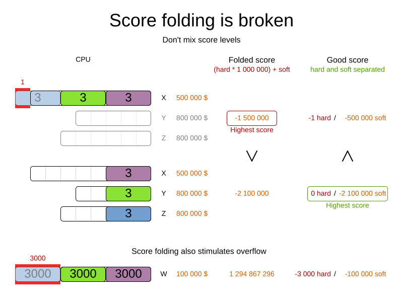
Your business might tell you that your hard constraints all have the same weight because they cannot be broken and therefore the weight does not matter. This is not true. If no feasible solution exists for a specific data set, the business can use the least infeasible solution to estimate how many business resources they are lacking. For example, in the cloud balancing problem, the least infeasible solution can reveal how many new computers are needed.
Furthermore, if all of your hard constraints have the same weight, you will likely create a score trap. For example, in the cloud balancing problem if a computer has seven too few CPUs for its processes, then it must be weighted seven times as much as if it had only one CPU too few.
OptaPlanner supports three or more score levels as well. For example, a company might decide that profit outranks employee satisfaction, or vice versa, while both constraints are outranked by the constraints of physical reality.
To model fairness or load balancing, you do not need to use lots of score levels even though OptaPlanner can handle many score levels.
Most use cases use a score with two or three weights, such as HardSoftScore and HardMediumSoftScore. You can combine all of these techniques seemlessly:
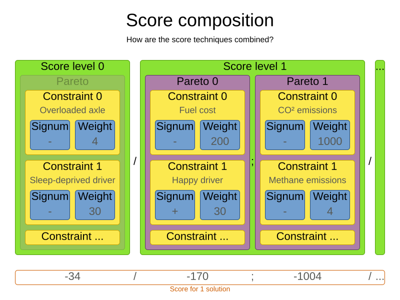
Chapter 10. The OptaPlanner Score interface
A score is represented by the Score interface, which extends the Comparable interface:
public interface Score<...> extends Comparable<...> {
    ...
}
public interface Score<...> extends Comparable<...> {
    ...
}
The score implementation to use depends on your use case. Your score might not efficiently fit in a single long value. OptaPlanner has several built-in score implementations, but you can implement a custom score as well. Most use cases use the built-in HardSoftScore score.

All Score implementations also have an initScore (which is an int). It is mostly intended for internal use in OptaPlanner: it is the negative number of uninitialized planning variables. From a user’s perspective, this is 0, unless a construction heuristic is terminated before it could initialize all planning variables. In this case, Score.isSolutionInitialized() returns false.
The score implementation (for example HardSoftScore) must be the same throughout a solver runtime. The score implementation is configured in the solution domain class:
10.1. Floating point numbers in score calculation
Avoid the use of the floating point number types float or double in score calculation. Use BigDecimal or scaled long instead. Floating point numbers cannot represent a decimal number correctly. For example, a double cannot contain the value 0.05 correctly. Instead, it contains the nearest representable value. Arithmetic, including addition and subtraction, that uses floating point numbers, especially for planning problems, leads to incorrect decisions as shown in the following illustration:

Additionally, floating point number addition is not associative:
System.out.println( ((0.01 + 0.02) + 0.03) == (0.01 + (0.02 + 0.03)) ); // returns false
System.out.println( ((0.01 + 0.02) + 0.03) == (0.01 + (0.02 + 0.03)) ); // returns falseThis leads to score corruption.
Decimal numbers (BigDecimal) have none of these problems.
BigDecimal arithmetic is considerably slower than int, long, or double arithmetic. In some experiments, the score calculation takes five times longer.
Therefore, in many cases, it can be worthwhile to multiply all numbers for a single score weight by a plural of ten, so the score weight fits in a scaled int or long. For example, if you multiply all weights by 1000, a fuelCost of 0.07 becomes a fuelCostMillis of 70 and no longer uses a decimal score weight.
10.2. Score calculation types
There are several types of ways to calculate the score of a solution:
- Easy Java score calculation: Implement all constraints together in a single method in Java or another JVM language. This method does not scale.
- Constraint streams score calculation: Implement each constraint as a separate constraint stream in Java or another JVM language. This method is fast and scalable.
- Incremental Java score calculation (not recommended): Implement multiple low-level methods in Java or another JVM language. This method is fast and scalable but very difficult to implement and maintain.
- Drools score calculation (deprecated): Implement each constraint as a separate score rule in DRL. This method is scalable.
Each score calculation type can work with any score definition, for example HardSoftScore or HardMediumSoftScore. All score calculation types are object oriented and can reuse existing Java code.
The score calculation must be read-only. It must not change the planning entities or the problem facts in any way. For example, the score calculation must not call a setter method on a planning entity in the score calculation.
OptaPlanner does not recalculate the score of a solution if it can predict it unless an environmentMode assertion is enabled. For example, after a winning step is done, there is no need to calculate the score because that move was done and undone earlier. As a result, there is no guarantee that changes applied during score calculation actually happen.
To update planning entities when the planning variable changes, use shadow variables instead.
10.2.1. Implenting the Easy Java score calculation type
The Easy Java score calculation type provides an easy way to implement your score calculation in Java. You can implement all constraints together in a single method in Java or another JVM language.
Advantages:
- Uses plain old Java so there is no learning curve
- Provides an opportunity to delegate score calculation to an existing code base or legacy system
Disadvantages:
- Slowest calculation type
- Does not scale because there is no incremental score calculation
Procedure
Implement the
EasyScoreCalculatorinterface:public interface EasyScoreCalculator<Solution_, Score_ extends Score<Score_>> { Score_ calculateScore(Solution_ solution); }public interface EasyScoreCalculator<Solution_, Score_ extends Score<Score_>> { Score_ calculateScore(Solution_ solution); }Copy to Clipboard Copied! Toggle word wrap Toggle overflow The following example implements this interface in the N Queens problem:
Copy to Clipboard Copied! Toggle word wrap Toggle overflow Configure the
EasyScoreCalculatorclass in the solver configuration. The following example shows how to implement this interface in the N Queens problem:<scoreDirectorFactory> <easyScoreCalculatorClass>org.optaplanner.examples.nqueens.optional.score.NQueensEasyScoreCalculator</easyScoreCalculatorClass> </scoreDirectorFactory><scoreDirectorFactory> <easyScoreCalculatorClass>org.optaplanner.examples.nqueens.optional.score.NQueensEasyScoreCalculator</easyScoreCalculatorClass> </scoreDirectorFactory>Copy to Clipboard Copied! Toggle word wrap Toggle overflow To configure values of the
EasyScoreCalculatormethod dynamically in the solver configuration so that the benchmarker can tweak those parameters, add theeasyScoreCalculatorCustomPropertieselement and use custom properties:Copy to Clipboard Copied! Toggle word wrap Toggle overflow
10.2.2. Implementing the Incremental Java score calculation type
The Incremental Java score calculation type provides a way to implement your score calculation incrementally in Java.
This type is not recommended.
Advantages:
- Very fast and scalable. This is currently the fastest type if implemented correctly.
Disadvantages:
Hard to write.
- A scalable implementation that heavily uses maps, indexes, and so forth.
- You have to learn, design, write, and improve all of these performance optimizations yourself.
- Hard to read. Regular score constraint changes can lead to a high maintenance cost.
Procedure
Implement all of the methods of the
IncrementalScoreCalculatorinterface:Copy to Clipboard Copied! Toggle word wrap Toggle overflow The following example implements this interface in the N Queens problem:
Copy to Clipboard Copied! Toggle word wrap Toggle overflow Configure the
incrementalScoreCalculatorClassclass in the solver configuration. The following example shows how to implement this interface in the N Queens problem:<scoreDirectorFactory> <incrementalScoreCalculatorClass>org.optaplanner.examples.nqueens.optional.score.NQueensAdvancedIncrementalScoreCalculator</incrementalScoreCalculatorClass> </scoreDirectorFactory><scoreDirectorFactory> <incrementalScoreCalculatorClass>org.optaplanner.examples.nqueens.optional.score.NQueensAdvancedIncrementalScoreCalculator</incrementalScoreCalculatorClass> </scoreDirectorFactory>Copy to Clipboard Copied! Toggle word wrap Toggle overflow ImportantA piece of incremental score calculator code can be difficult to write and to review. Assert its correctness by using an
EasyScoreCalculatorto fulfill the assertions triggered by theenvironmentMode.To configure values of an
IncrementalScoreCalculatordynamically in the solver configuration so the benchmarker can tweak those parameters, add theincrementalScoreCalculatorCustomPropertieselement and use custom properties:Copy to Clipboard Copied! Toggle word wrap Toggle overflow Optional: Implement the
ConstraintMatchAwareIncrementalScoreCalculatorinterface to facilitate the following goals:-
Explain a score by splitting it up for each score constraint with
ScoreExplanation.getConstraintMatchTotalMap(). -
Visualize or sort planning entities by how many constraints each one breaks with
ScoreExplanation.getIndictmentMap(). Receive a detailed analysis if the
IncrementalScoreCalculatoris corrupted inFAST_ASSERTorFULL_ASSERTenvironmentMode.Copy to Clipboard Copied! Toggle word wrap Toggle overflow For example, in machine reassignment create one
ConstraintMatchTotalfor each constraint type and calladdConstraintMatch()for each constraint match:Copy to Clipboard Copied! Toggle word wrap Toggle overflow The
getConstraintMatchTotals()code often duplicates some of the logic of the normalIncrementalScoreCalculatormethods. Constraint Streams and Drools Score Calculation do not have this disadvantage because they are constraint-match aware automatically when needed without any extra domain-specific code.
-
Explain a score by splitting it up for each score constraint with

Chapter 11. The InitializingScoreTrend class
You can add the InitializingScoreTrend class to optimization algorithms to specify how the score changes when additional variables are initialized and the already-initialized variables do not change. Some optimization algorithms, such Construction Heuristics and Exhaustive Search, run faster when this information is available.
You can specify one of the following trends for the score or each score level separately:
-
ANY(default): Initializing an extra variable can change the score positively or negatively. This trend does not provide a performance gain. ONLY_UP(rare): Initializing an extra variable can only change the score positively. TheONLY_UPtrend requires the following conditions:- There are only positive constraints.
- Initializing the next variable cannot unmatch a positive constraint that was matched by a previous initialized variable.
ONLY_DOWN: Initializing an additional variable can only change the score negatively.ONLY_DOWNrequires the following conditions:- There are only negative constraints.
- Initializing the next variable cannot unmatch a negative constraint that was matched by a previous initialized variable.
Most use cases have only negative constraints. Many of those use cases have an InitializingScoreTrend class that only goes down, as shown in the following example:
  <scoreDirectorFactory>
    <constraintProviderClass>org.optaplanner.examples.cloudbalancing.score.CloudBalancingConstraintProvider</constraintProviderClass>
    <initializingScoreTrend>ONLY_DOWN</initializingScoreTrend>
  </scoreDirectorFactory>
  <scoreDirectorFactory>
    <constraintProviderClass>org.optaplanner.examples.cloudbalancing.score.CloudBalancingConstraintProvider</constraintProviderClass>
    <initializingScoreTrend>ONLY_DOWN</initializingScoreTrend>
</scoreDirectorFactory>Alternatively, you can also specify the trend for each score level separately, as shown in the following example:
  <scoreDirectorFactory>
    <constraintProviderClass>org.optaplanner.examples.cloudbalancing.score.CloudBalancingConstraintProvider</constraintProviderClass>
    <initializingScoreTrend>ONLY_DOWN/ONLY_DOWN</initializingScoreTrend>
  </scoreDirectorFactory>
  <scoreDirectorFactory>
    <constraintProviderClass>org.optaplanner.examples.cloudbalancing.score.CloudBalancingConstraintProvider</constraintProviderClass>
    <initializingScoreTrend>ONLY_DOWN/ONLY_DOWN</initializingScoreTrend>
</scoreDirectorFactory>Chapter 12. Invalid score detection
If you use the environmentMode class and specify the value as FULL_ASSERT or FAST_ASSERT, the environment mode detects score corruption in the incremental score calculation.
However, doing this will not verify that your score calculator implements your score constraints the way that your business wants. For example, one constraint might consistently match the wrong pattern. To verify the constraints against an independent implementation, configure an assertionScoreDirectorFactory class:
In this example, the NQueensConstraintProvider implementation is validated by the EasyScoreCalculator.
This technique works well to isolate score corruption, but to verify that the constraint implements the real business needs, a unit test with a ConstraintVerifier is usually better.
Chapter 13. Score calculation performance tricks
Most of the execution time of a solver involves running the score calculation, which is called in the solver’s deepest loops. Faster score calculation returns the same solution in less time with the same algorithm. This usually provides a better solution in the same amount of time. Use the following techniques to improve your score calculation performance.
13.1. Score calculation speed
When you are improving your score calculation, focus on maximizing the score calculation speed instead of maximizing the best score. A big improvement in score calculation can sometimes yield little or no best score improvement, for example when the algorithm is stuck in a local or global optima. If you are watching the calculation speed instead, score calculation improvements are far more visible.
The score calculation speed per second is a reliable measurement of score calculation performance, even though it is affected by non-score calculation execution time. The result depends on the problem scale of the problem data set. Normally, even for high scale problems, the score calculation speed per second is higher than 1000, unless you are using an EasyScoreCalculator class.
By watching the calculation speed, you can remove or add score constraints and compare the latest calculation speed with the original calculation speed.
Comparing the best score with the original best score is pointless. It’s like comparing apples and oranges.
13.2. Incremental score calculation
Incremental score calculation is also known as delta-based score calculation. When a solution changes, incremental score calculation finds the new score by evaluating changes between the current state and the previous state instead of recalculating the entire score on every solution evaluation. For example, in the N Queens problem, when queen A moves from row 1 to 2, the incrementalScoreCalculation class does not check whether queen B and C can attack each other, because neither of them changed position, as shown in the following illustration:

The following example show incremental score calculation for employee rostering:

Incremental score calculation provides a significant performance and scalability gain. Constraint streams or Drools score calculation provides this scalability gain without forcing you to write a complicated incremental score calculation algorithm. Just let the rule engine do the hard work.
Notice that the increase in calculation speed is relative to the size of your planning problem (your n). This makes incremental score calculation scalable.
13.3. Remote services
Do not call remote services in your score calculation unless you are bridging the EasyScoreCalculator class to a legacy system. The network latency will significantly downgrade your score calculation performance. Cache the results of those remote services if possible.
If some parts of a constraint can be calculated once, when the solver starts, and never change during solving, then turn them into cached problem facts.
13.4. Pointless constraints
If you know that a specific constraint can never be broken or that it is always broken, do not write a score constraint for it. For example, in the N Queens problem, the score calculation does not check whether multiple queens occupy the same column because a queen’s column never changes and every solution starts with each queen on a different column.
Do not overuse this technique. If some data sets do not use a specific constraint but others do, just return out of the constraint as soon as you can. There is no need to dynamically change your score calculation based on the data set.
13.5. Built-in hard constraints
Instead of implementing a hard constraint, the hard constraint can sometimes be built in. For example, in the school timetabling example, if Lecture A should never be assigned to Room X, but it uses the ValueRangeProvider class on Solution, the Solver will often try to assign it to Room X only to discover that it breaks a hard constraint. Use a ValueRangeProvider on the planning entity or filtered selection to define that Lecture A should only be assigned a Room different than X.
This can give a good performance gain in some use cases, not just because the score calculation is faster, but because most optimization algorithms will spend less time evaluating infeasible solutions. However, usually this is not a good idea because there is a real risk of trading short term benefits for long term harm:
- Many optimization algorithms rely on the freedom to break hard constraints when changing planning entities, to get out of local optima.
- Both implementation approaches have limitations such as feature compatibility and disabling automatic performance optimizations.
13.6. Score traps
Make sure that none of your score constraints cause a score trap. A trapped score constraint applies the same weight to multiple constraint matches. Doing this groups constraint matches together and creates a flatlined score function for that constraint. This can cause a solution state in which several moves must be done to resolve or lower the weight of that single constraint. The following examples illustrate score traps:
- You need two doctors at each operating table but you are only moving one doctor at a time. The solver has no incentive to move a doctor to a table with no doctors. To fix this, penalize a table with no doctors more than a table with only one doctor in that score constraint in the score function.
- Two exams must be conducted at the same time, but you are only moving one exam at a time. The solver must move one of those exams to another time slot without moving the other in the same move. To fix this, add a coarse-grained move that moves both exams at the same time.
The following illustration shows a score trap:

If the blue item moves from an overloaded computer to an empty computer, the hard score should improve. But the trapped score implementation cannot do that. The solver should eventually get out of this trap, but it will take a lot of effort, especially if there are even more processes on the overloaded computer. Before it can do that, it might actually start moving more processes into that overloaded computer, because there is no penalty for doing so.
Avoiding score traps does not mean that your score function should be smart enough to avoid local optima. Leave it to the optimization algorithms to deal with the local optima.
Avoiding score traps means to avoid, for each score constraint individually, a flatlined score function.
Always specify the degree of infeasibility. The business often says "if the solution is infeasible, it does not matter how infeasible it is." While that is true for the business, it is not true for score calculation because score calculation benefits from knowing how infeasible a solution is. In practice, soft constraints usually do this naturally and it is just a matter of doing it for the hard constraints too.
There are several ways to deal with a score trap:
-
Improve the score constraint to make a distinction in the score weight. For example, penalize
-1hardfor every missing CPU instead of just-1hardif any CPU is missing. -
If changing the score constraint is not allowed from the business perspective, add a lower score level with a score constraint that makes such a distinction. For example, penalize
-1subsoftfor every missing CPU, on top of-1hardif any CPU is missing. The business ignores the subsoft score level. - Add coarse-grained moves and union-select them with the existing fine-grained moves. A coarse-grained move effectively does multiple moves to directly get out of a score trap with a single move. For example, move multiple items from the same container to another container.
13.7. The stepLimit benchmark
Not all score constraints have the same performance cost. Sometimes one score constraint can kill the score calculation performance outright. Use the benchmarker to perform a one minute run and then check what happens to the score calculation speed if you comment out all but one of the score constraints.
13.8. Fairness score constraints
Some use cases have a business requirement to provide a fair schedule, usually as a soft score constraint, for example:
- To avoid envy, fairly distribute the workload among the employees.
- To improve reliability, evenly distribute the workload among assets.
Implementing such a constraint might seem difficult, especially because there are different ways to formalize fairness, but usually the squared workload implementation behaves in the most desirable manner. For each employee or asset, specify the workload as w and subtract w² from the score.

The squared workload implementation guarantees that if you select two employees from a specified solution and make the distribution between those two employees fairer, then the resulting new solution will have a better overall score. Do not use only the difference from the average workload because that can lead to unfairness, as demonstrated in the following illustration:

Instead of the squared workload implementation, it is also possible to use the variance (squared difference to the average) or the standard deviation (square root of the variance). This has no effect on the score comparison, because the average does not change during planning. It is just more work to implement because the average needs to be known and trivially slower because the calculation takes a little longer.
When the workload is perfectly balanced, users often like to see a 0 score, instead of the distracting -34soft. This is shown in the preceding image for the last solution which is almost perfectly balanced. To nullify this, either add the average multiplied by the number of entities to the score or show the variance or standard deviation in the UI.
13.9. Other score calculation performance tricks
Use the following tips to further improve your score calculation performance:
-
Verify that your score calculation occurs in the correct number type. For example, if you are adding values of the type
int, do not store the result as the typedouble, which takes longer to calculate. - For optimal performance, use the latest Java version. For example, you can achieve a ~10 % performance increase by switching from Java 11 to 17.
- Always remember that premature optimization is very undesireable. Make sure your design is flexible enough to allow configuration-based adjustments.
13.10. Configuing constraints
Deciding the correct weight and level for each constraint is not easy. It often involves negotiating with different stakeholders and their priorities. Furthermore, quantifying the impact of soft constraints is often a new experience for business managers, so they need a number of iterations to get it right. To make this easier, use the @ConstraintConfiguration class with constraint weights and parameters. Then, provide a UI so business managers can adjust the constraint weights themselves and visualize the resulting solution, as shown in the following illustration:

For example, in the conference scheduling problem, the minimum pause constraint has a constraint weight, but it also has a constraint parameter that defines the length of time between two talks by the same speaker. The pause length depends on the conference: in some large conferences 20 minutes isn’t enough time to go from one room to the other and in smaller conferences 10 minutes can be enough time. The pause length is a field in the constraint configuration without a @ConstraintWeight annotation.
Each constraint has a constraint package and a constraint name and together they form the constraint ID. The constraint ID connects the constraint weight with the constraint implementation. For each constraint weight, there must be a constraint implementation with the same package and the same name.
-
The
@ConstraintConfigurationannotation has aconstraintPackageproperty that defaults to the package of the constraint configuration class. Cases with constraint streams normally do not need to specify it. -
The
@ConstraintWeightannotation has avaluewhich is the constraint name (for example "Speaker conflict"). It inherits the constraint package from the@ConstraintConfiguration, but it can override that, for example@ConstraintWeight(constraintPackage = "…region.france", …)to use a different constraint package than some other weights.
So every constraint weight ends up with a constraint package and a constraint name. Each constraint weight links with a constraint implementation, for example in constraint streams:
Each of the constraint weights defines the score level and score weight of their constraint. The constraint implementation calls rewardConfigurable() or penalizeConfigurable() and the constraint weight is automatically applied.
If the constraint implementation provides a match weight, that match weight is multiplied with the constraint weight. For example, the content conflict constraint weight defaults to 100soft and the constraint implementation penalizes each match based on the number of shared content tags and the overlapping duration of the two talks:
    @ConstraintWeight("Content conflict")
    private HardMediumSoftScore contentConflict = HardMediumSoftScore.ofSoft(100);
    @ConstraintWeight("Content conflict")
    private HardMediumSoftScore contentConflict = HardMediumSoftScore.ofSoft(100);
So when 2 overlapping talks share only 1 content tag and overlap by 60 minutes, the score is impacted by -6000soft. But when 2 overlapping talks share 3 content tags, the match weight is 180, so the score is impacted by -18000soft.
Procedure
-
Create a new class to hold the constraint weights and other constraint parameters, for example
ConferenceConstraintConfiguration. Annotate this class with
@ConstraintConfiguration:@ConstraintConfiguration public class ConferenceConstraintConfiguration { ... }@ConstraintConfiguration public class ConferenceConstraintConfiguration { ... }Copy to Clipboard Copied! Toggle word wrap Toggle overflow Add the constraint configuration on the planning solution and annotate that field or property with
@ConstraintConfigurationProvider:Copy to Clipboard Copied! Toggle word wrap Toggle overflow In the constraint configuration class, add a
@ConstraintWeightproperty for each constraint and give each constraint weight a default value:Copy to Clipboard Copied! Toggle word wrap Toggle overflow The
@ConstraintConfigurationProviderannotation automatically exposes the constraint configuration as a problem fact. There is no need to add a@ProblemFactPropertyannotation. A constraint weight cannot be null.-
Expose the constraint weights in a UI so business users can tweak the values. The preceding example uses the
ofHard(),ofMedium()andofSoft()methods to do that. Notice how it defaults the content conflict constraint as ten times more important than the theme track conflict constraint. Normally, a constraint weight only uses one score level, but it’s possible to use multiple score levels (at a small performance cost).
13.11. Explaining the score
There are several ways to show how the OptaPlanner score is derived. This is called explaining the score:
-
Print the return value of
getSummary(). This is the easiest way to explain the score during development, but only use this method for diagnostic purposes. -
Use the
ScoreManagerAPI in an application or web UI. Break down the score for each constraint for a more granular view.

Procedure
Use one of the following methods to explain the score:
Print the return value of
getSummary():System.out.println(scoreManager.getSummary(solution));
System.out.println(scoreManager.getSummary(solution));Copy to Clipboard Copied! Toggle word wrap Toggle overflow The following conference scheduling example prints that talk
S51is responsible for breaking the hard constraintSpeaker required room tag:Copy to Clipboard Copied! Toggle word wrap Toggle overflow ImportantDo not attempt to parse this string or use it in your UI or exposed services. Instead use the ConstraintMatch API.
Use the
ScoreManagerAPI in an application or web UI.Enter code similar to the following example:
ScoreManager<CloudBalance, HardSoftScore> scoreManager = ScoreManager.create(solverFactory);
ScoreExplanation<CloudBalance, HardSoftScore> scoreExplanation = scoreManager.explainScore(cloudBalance);
ScoreManager<CloudBalance, HardSoftScore> scoreManager = ScoreManager.create(solverFactory);
ScoreExplanation<CloudBalance, HardSoftScore> scoreExplanation = scoreManager.explainScore(cloudBalance);
Copy to Clipboard Copied! Toggle word wrap Toggle overflow Use this code when you need to calculate the score of a solution:
HardSoftScore score = scoreExplanation.getScore();
HardSoftScore score = scoreExplanation.getScore();Copy to Clipboard Copied! Toggle word wrap Toggle overflow
Break down the score by constraint:
Get the
ConstraintMatchTotalvalues fromScoreExplanation:Copy to Clipboard Copied! Toggle word wrap Toggle overflow Each
ConstraintMatchTotalrepresents one constraint and has a part of the overall score. The sum of all theConstraintMatchTotal.getScore()equals the overall score.NoteConstraint streams and Drools score calculation support constraint matches automatically, but incremental Java score calculation requires implementing an extra interface.
13.12. Visualizing the hot planning entities
Show a heat map in the UI that highlights the planning entities and problem facts that have an impact on the score.
Procedure
Get the
Indictmentmap from theScoreExplanation:Copy to Clipboard Copied! Toggle word wrap Toggle overflow Each
Indictmentis the sum of all constraints where that justification object is involved. The sum of all theIndictment.getScoreTotal()differs from the overall score because multipleIndictmententities can share the sameConstraintMatch.NoteConstraint streams and Drools score calculation supports constraint matches automatically, but incremental Java score calculation requires implementing an extra interface.
13.13. Score constraints testing
Different score calculation types come with different tools for testing. Write a unit test for each score constraint individually to check that it behaves correctly.
Part V. Red Hat Build of OptaPlanner quick start guides
Red Hat Build of OptaPlanner provides the following quick start guides to demonstrate how OptaPlanner can integrate with different techologies:
- Red Hat Build of OptaPlanner on the Red Hat build of Quarkus platform: a school timetable quick start guide
- Red Hat Build of OptaPlanner on the Red Hat build of Quarkus platform: a vaccination appointment scheduler quick start guide
- Red Hat Build of OptaPlanner on the Red Hat build of Quarkus platform: an employee scheduler quick start guide
- Red Hat Build of OptaPlanner on Spring Boot: a school timetable quick start guide
- Red Hat Build of OptaPlanner with Java solvers: a school timetable quick start guide
Chapter 14. Red Hat Build of OptaPlanner on the Red Hat build of Quarkus platform: a school timetable quick start guide
This guide walks you through the process of creating a Red Hat build of Quarkus application using the Red Hat Build of OptaPlanner constraint solving artificial intelligence (AI). You will build a REST application that optimizes a school timetable for students and teachers
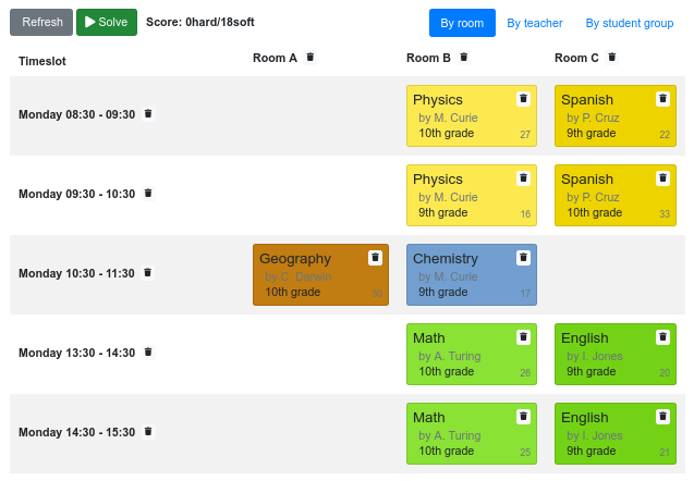
Your service will assign Lesson instances to Timeslot and Room instances automatically by using AI to adhere to the following hard and soft scheduling constraints:
- A room can have at most one lesson at the same time.
- A teacher can teach at most one lesson at the same time.
- A student can attend at most one lesson at the same time.
- A teacher prefers to teach in a single room.
- A teacher prefers to teach sequential lessons and dislikes gaps between lessons.
Mathematically speaking, school timetabling is an NP-hard problem. That means it is difficult to scale. Simply iterating through all possible combinations with brute force would take millions of years for a non-trivial data set, even on a supercomputer. Fortunately, AI constraint solvers such as Red Hat Build of OptaPlanner have advanced algorithms that deliver a near-optimal solution in a reasonable amount of time. What is considered to be a reasonable amount of time is subjective and depends on the goals of your problem.
Prerequisites
- OpenJDK 11 or later is installed. Red Hat build of Open JDK is available from the Software Downloads page in the Red Hat Customer Portal (login required).
- Apache Maven 3.8 or higher is installed. Maven is available from the Apache Maven Project website.
- An IDE, such as IntelliJ IDEA, VSCode, or Eclipse is available.
- An Red Hat Build of OptaPlanner Red Hat build of Quarkus project is available. For instruction on creating an Red Hat Build of OptaPlanner Red Hat build of Quarkus project, see "Getting started with OptaPlanner and Quarkus" in the Getting Started with Red Hat Build of OptaPlanner section.
14.1. Model the domain objects
The goal of the Red Hat Build of OptaPlanner timetable project is to assign each lesson to a time slot and a room. To do this, add three classes, Timeslot, Lesson, and Room, as shown in the following diagram:

Timeslot
The Timeslot class represents a time interval when lessons are taught, for example, Monday 10:30 - 11:30 or Tuesday 13:30 - 14:30. In this example, all time slots have the same duration and there are no time slots during lunch or other breaks.
A time slot has no date because a high school schedule just repeats every week. There is no need for continuous planning. A timeslot is called a problem fact because no Timeslot instances change during solving. Such classes do not require any OptaPlanner-specific annotations.
Room
The Room class represents a location where lessons are taught, for example, Room A or Room B. In this example, all rooms are without capacity limits and they can accommodate all lessons.
Room instances do not change during solving so Room is also a problem fact.
Lesson
During a lesson, represented by the Lesson class, a teacher teaches a subject to a group of students, for example, Math by A.Turing for 9th grade or Chemistry by M.Curie for 10th grade. If a subject is taught multiple times each week by the same teacher to the same student group, there are multiple Lesson instances that are only distinguishable by id. For example, the 9th grade has six math lessons a week.
During solving, OptaPlanner changes the timeslot and room fields of the Lesson class to assign each lesson to a time slot and a room. Because OptaPlanner changes these fields, Lesson is a planning entity:

Most of the fields in the previous diagram contain input data, except for the orange fields. A lesson’s timeslot and room fields are unassigned (null) in the input data and assigned (not null) in the output data. OptaPlanner changes these fields during solving. Such fields are called planning variables. In order for OptaPlanner to recognize them, both the timeslot and room fields require an @PlanningVariable annotation. Their containing class, Lesson, requires an @PlanningEntity annotation.
Procedure
Create the
src/main/java/com/example/domain/Timeslot.javaclass:Copy to Clipboard Copied! Toggle word wrap Toggle overflow Notice the
toString()method keeps the output short so it is easier to read OptaPlanner’sDEBUGorTRACElog, as shown later.Create the
src/main/java/com/example/domain/Room.javaclass:Copy to Clipboard Copied! Toggle word wrap Toggle overflow Create the
src/main/java/com/example/domain/Lesson.javaclass:Copy to Clipboard Copied! Toggle word wrap Toggle overflow The
Lessonclass has an@PlanningEntityannotation, so OptaPlanner knows that this class changes during solving because it contains one or more planning variables.The
timeslotfield has an@PlanningVariableannotation, so OptaPlanner knows that it can change its value. In order to find potentialTimeslotinstances to assign to this field, OptaPlanner uses thevalueRangeProviderRefsproperty to connect to a value range provider that provides aList<Timeslot>to pick from. See Section 14.3, “Gather the domain objects in a planning solution” for information about value range providers.The
roomfield also has an@PlanningVariableannotation for the same reasons.
14.2. Define the constraints and calculate the score
When solving a problem, a score represents the quality of a specific solution. The higher the score the better. Red Hat Build of OptaPlanner looks for the best solution, which is the solution with the highest score found in the available time. It might be the optimal solution.
Because the timetable example use case has hard and soft constraints, use the HardSoftScore class to represent the score:
- Hard constraints must not be broken. For example: A room can have at most one lesson at the same time.
- Soft constraints should not be broken. For example: A teacher prefers to teach in a single room.
Hard constraints are weighted against other hard constraints. Soft constraints are weighted against other soft constraints. Hard constraints always outweigh soft constraints, regardless of their respective weights.
To calculate the score, you could implement an EasyScoreCalculator class:
Unfortunately, this solution does not scale well because it is non-incremental: every time a lesson is assigned to a different time slot or room, all lessons are re-evaluated to calculate the new score.
A better solution is to create a src/main/java/com/example/solver/TimeTableConstraintProvider.java class to perform incremental score calculation. This class uses OptaPlanner’s ConstraintStream API which is inspired by Java 8 Streams and SQL. The ConstraintProvider scales an order of magnitude better than the EasyScoreCalculator: O(n) instead of O(n²).
Procedure
Create the following src/main/java/com/example/solver/TimeTableConstraintProvider.java class:
14.3. Gather the domain objects in a planning solution
A TimeTable instance wraps all Timeslot, Room, and Lesson instances of a single dataset. Furthermore, because it contains all lessons, each with a specific planning variable state, it is a planning solution and it has a score:
-
If lessons are still unassigned, then it is an uninitialized solution, for example, a solution with the score
-4init/0hard/0soft. -
If it breaks hard constraints, then it is an infeasible solution, for example, a solution with the score
-2hard/-3soft. -
If it adheres to all hard constraints, then it is a feasible solution, for example, a solution with the score
0hard/-7soft.
The TimeTable class has an @PlanningSolution annotation, so Red Hat Build of OptaPlanner knows that this class contains all of the input and output data.
Specifically, this class is the input of the problem:
A
timeslotListfield with all time slots- This is a list of problem facts, because they do not change during solving.
A
roomListfield with all rooms- This is a list of problem facts, because they do not change during solving.
A
lessonListfield with all lessons- This is a list of planning entities because they change during solving.
Of each
Lesson:-
The values of the
timeslotandroomfields are typically stillnull, so unassigned. They are planning variables. -
The other fields, such as
subject,teacherandstudentGroup, are filled in. These fields are problem properties.
-
The values of the
However, this class is also the output of the solution:
-
A
lessonListfield for which eachLessoninstance has non-nulltimeslotandroomfields after solving -
A
scorefield that represents the quality of the output solution, for example,0hard/-5soft
Procedure
Create the src/main/java/com/example/domain/TimeTable.java class:
The value range providers
The timeslotList field is a value range provider. It holds the Timeslot instances which OptaPlanner can pick from to assign to the timeslot field of Lesson instances. The timeslotList field has an @ValueRangeProvider annotation to connect those two, by matching the id with the valueRangeProviderRefs of the @PlanningVariable in the Lesson.
Following the same logic, the roomList field also has an @ValueRangeProvider annotation.
The problem fact and planning entity properties
Furthermore, OptaPlanner needs to know which Lesson instances it can change as well as how to retrieve the Timeslot and Room instances used for score calculation by your TimeTableConstraintProvider.
The timeslotList and roomList fields have an @ProblemFactCollectionProperty annotation, so your TimeTableConstraintProvider can select from those instances.
The lessonList has an @PlanningEntityCollectionProperty annotation, so OptaPlanner can change them during solving and your TimeTableConstraintProvider can select from those too.
14.4. Create the solver service
Solving planning problems on REST threads causes HTTP timeout issues. Therefore, the Quarkus extension injects a SolverManager, which runs solvers in a separate thread pool and can solve multiple data sets in parallel.
Procedure
Create the src/main/java/org/acme/optaplanner/rest/TimeTableResource.java class:
This initial implementation waits for the solver to finish, which can still cause an HTTP timeout. The complete implementation avoids HTTP timeouts much more elegantly.
14.5. Set the solver termination time
If your planning application does not have a termination setting or a termination event, it theoretically runs forever and in reality eventually causes an HTTP timeout error. To prevent this from occurring, use the optaplanner.solver.termination.spent-limit parameter to specify the length of time after which the application terminates. In most applications, set the time to at least five minutes (5m). However, in the Timetable example, limit the solving time to five seconds, which is short enough to avoid the HTTP timeout.
Procedure
Create the src/main/resources/application.properties file with the following content:
quarkus.optaplanner.solver.termination.spent-limit=5s
quarkus.optaplanner.solver.termination.spent-limit=5s14.6. Running the school timetable application
After you have created the school timetable project, run it in development mode. In development mode, you can update the application sources and configurations while your application is running. Your changes will appear in the running application.
Prerequisites
- You have created the school timetable project.
Procedure
To compile the application in development mode, enter the following command from the project directory:
./mvnw compile quarkus:dev
./mvnw compile quarkus:devCopy to Clipboard Copied! Toggle word wrap Toggle overflow Test the REST service. You can use any REST client. The following example uses the Linux command
curlto send a POST request:curl -i -X POST http://localhost:8080/timeTable/solve -H "Content-Type:application/json" -d '{"timeslotList":[{"dayOfWeek":"MONDAY","startTime":"08:30:00","endTime":"09:30:00"},{"dayOfWeek":"MONDAY","startTime":"09:30:00","endTime":"10:30:00"}],"roomList":[{"name":"Room A"},{"name":"Room B"}],"lessonList":[{"id":1,"subject":"Math","teacher":"A. Turing","studentGroup":"9th grade"},{"id":2,"subject":"Chemistry","teacher":"M. Curie","studentGroup":"9th grade"},{"id":3,"subject":"French","teacher":"M. Curie","studentGroup":"10th grade"},{"id":4,"subject":"History","teacher":"I. Jones","studentGroup":"10th grade"}]}'$ curl -i -X POST http://localhost:8080/timeTable/solve -H "Content-Type:application/json" -d '{"timeslotList":[{"dayOfWeek":"MONDAY","startTime":"08:30:00","endTime":"09:30:00"},{"dayOfWeek":"MONDAY","startTime":"09:30:00","endTime":"10:30:00"}],"roomList":[{"name":"Room A"},{"name":"Room B"}],"lessonList":[{"id":1,"subject":"Math","teacher":"A. Turing","studentGroup":"9th grade"},{"id":2,"subject":"Chemistry","teacher":"M. Curie","studentGroup":"9th grade"},{"id":3,"subject":"French","teacher":"M. Curie","studentGroup":"10th grade"},{"id":4,"subject":"History","teacher":"I. Jones","studentGroup":"10th grade"}]}'Copy to Clipboard Copied! Toggle word wrap Toggle overflow After the time period specified in
termination spent timedefined in yourapplication.propertiesfile, the service returns output similar to the following example:HTTP/1.1 200 Content-Type: application/json ... {"timeslotList":...,"roomList":...,"lessonList":[{"id":1,"subject":"Math","teacher":"A. Turing","studentGroup":"9th grade","timeslot":{"dayOfWeek":"MONDAY","startTime":"08:30:00","endTime":"09:30:00"},"room":{"name":"Room A"}},{"id":2,"subject":"Chemistry","teacher":"M. Curie","studentGroup":"9th grade","timeslot":{"dayOfWeek":"MONDAY","startTime":"09:30:00","endTime":"10:30:00"},"room":{"name":"Room A"}},{"id":3,"subject":"French","teacher":"M. Curie","studentGroup":"10th grade","timeslot":{"dayOfWeek":"MONDAY","startTime":"08:30:00","endTime":"09:30:00"},"room":{"name":"Room B"}},{"id":4,"subject":"History","teacher":"I. Jones","studentGroup":"10th grade","timeslot":{"dayOfWeek":"MONDAY","startTime":"09:30:00","endTime":"10:30:00"},"room":{"name":"Room B"}}],"score":"0hard/0soft"}HTTP/1.1 200 Content-Type: application/json ... {"timeslotList":...,"roomList":...,"lessonList":[{"id":1,"subject":"Math","teacher":"A. Turing","studentGroup":"9th grade","timeslot":{"dayOfWeek":"MONDAY","startTime":"08:30:00","endTime":"09:30:00"},"room":{"name":"Room A"}},{"id":2,"subject":"Chemistry","teacher":"M. Curie","studentGroup":"9th grade","timeslot":{"dayOfWeek":"MONDAY","startTime":"09:30:00","endTime":"10:30:00"},"room":{"name":"Room A"}},{"id":3,"subject":"French","teacher":"M. Curie","studentGroup":"10th grade","timeslot":{"dayOfWeek":"MONDAY","startTime":"08:30:00","endTime":"09:30:00"},"room":{"name":"Room B"}},{"id":4,"subject":"History","teacher":"I. Jones","studentGroup":"10th grade","timeslot":{"dayOfWeek":"MONDAY","startTime":"09:30:00","endTime":"10:30:00"},"room":{"name":"Room B"}}],"score":"0hard/0soft"}Copy to Clipboard Copied! Toggle word wrap Toggle overflow Notice that your application assigned all four lessons to one of the two time slots and one of the two rooms. Also notice that it conforms to all hard constraints. For example, M. Curie’s two lessons are in different time slots.
To review what OptaPlanner did during the solving time, review the info log on the server side. The following is sample info log output:
... Solving started: time spent (33), best score (-8init/0hard/0soft), environment mode (REPRODUCIBLE), random (JDK with seed 0). ... Construction Heuristic phase (0) ended: time spent (73), best score (0hard/0soft), score calculation speed (459/sec), step total (4). ... Local Search phase (1) ended: time spent (5000), best score (0hard/0soft), score calculation speed (28949/sec), step total (28398). ... Solving ended: time spent (5000), best score (0hard/0soft), score calculation speed (28524/sec), phase total (2), environment mode (REPRODUCIBLE).
... Solving started: time spent (33), best score (-8init/0hard/0soft), environment mode (REPRODUCIBLE), random (JDK with seed 0). ... Construction Heuristic phase (0) ended: time spent (73), best score (0hard/0soft), score calculation speed (459/sec), step total (4). ... Local Search phase (1) ended: time spent (5000), best score (0hard/0soft), score calculation speed (28949/sec), step total (28398). ... Solving ended: time spent (5000), best score (0hard/0soft), score calculation speed (28524/sec), phase total (2), environment mode (REPRODUCIBLE).Copy to Clipboard Copied! Toggle word wrap Toggle overflow
14.7. Testing the application
A good application includes test coverage. Test the constraints and the solver in your timetable project.
14.7.1. Test the school timetable constraints
To test each constraint of the timetable project in isolation, use a ConstraintVerifier in unit tests. This tests each constraint’s corner cases in isolation from the other tests, which lowers maintenance when adding a new constraint with proper test coverage.
This test verifies that the constraint TimeTableConstraintProvider::roomConflict, when given three lessons in the same room and two of the lessons have the same timeslot, penalizes with a match weight of 1. So if the constraint weight is 10hard it reduces the score by -10hard.
Procedure
Create the src/test/java/org/acme/optaplanner/solver/TimeTableConstraintProviderTest.java class:
Notice how ConstraintVerifier ignores the constraint weight during testing even if those constraint weights are hardcoded in the ConstraintProvider. This is because constraint weights change regularly before going into production. This way, constraint weight tweaking does not break the unit tests.
14.7.2. Test the school timetable solver
This example tests the Red Hat Build of OptaPlanner school timetable project on the Red Hat build of Quarkus platform. It uses a JUnit test to generate a test data set and send it to the TimeTableController to solve.
Procedure
Create the
src/test/java/com/example/rest/TimeTableResourceTest.javaclass with the following content:Copy to Clipboard Copied! Toggle word wrap Toggle overflow This test verifies that after solving, all lessons are assigned to a time slot and a room. It also verifies that it found a feasible solution (no hard constraints broken).
Add test properties to the
src/main/resources/application.propertiesfile:Copy to Clipboard Copied! Toggle word wrap Toggle overflow
Normally, the solver finds a feasible solution in less than 200 milliseconds. Notice how the application.properties file overwrites the solver termination during tests to terminate as soon as a feasible solution (0hard/*soft) is found. This avoids hard coding a solver time, because the unit test might run on arbitrary hardware. This approach ensures that the test runs long enough to find a feasible solution, even on slow systems. But it does not run a millisecond longer than it strictly must, even on fast systems.
14.8. Logging
After you complete the Red Hat Build of OptaPlanner school timetable project, you can use logging information to help you fine-tune the constraints in the ConstraintProvider. Review the score calculation speed in the info log file to assess the impact of changes to your constraints. Run the application in debug mode to show every step that your application takes or use trace logging to log every step and every move.
Procedure
- Run the school timetable application for a fixed amount of time, for example, five minutes.
Review the score calculation speed in the
logfile as shown in the following example:... Solving ended: ..., score calculation speed (29455/sec), ...
... Solving ended: ..., score calculation speed (29455/sec), ...Copy to Clipboard Copied! Toggle word wrap Toggle overflow -
Change a constraint, run the planning application again for the same amount of time, and review the score calculation speed recorded in the
logfile. Run the application in debug mode to log every step that the application makes:
-
To run debug mode from the command line, use the
-Dsystem property. To permanently enable debug mode, add the following line to the
application.propertiesfile:quarkus.log.category."org.optaplanner".level=debug
quarkus.log.category."org.optaplanner".level=debugCopy to Clipboard Copied! Toggle word wrap Toggle overflow The following example shows output in the
logfile in debug mode:... Solving started: time spent (67), best score (-20init/0hard/0soft), environment mode (REPRODUCIBLE), random (JDK with seed 0). ... CH step (0), time spent (128), score (-18init/0hard/0soft), selected move count (15), picked move ([Math(101) {null -> Room A}, Math(101) {null -> MONDAY 08:30}]). ... CH step (1), time spent (145), score (-16init/0hard/0soft), selected move count (15), picked move ([Physics(102) {null -> Room A}, Physics(102) {null -> MONDAY 09:30}]). ...... Solving started: time spent (67), best score (-20init/0hard/0soft), environment mode (REPRODUCIBLE), random (JDK with seed 0). ... CH step (0), time spent (128), score (-18init/0hard/0soft), selected move count (15), picked move ([Math(101) {null -> Room A}, Math(101) {null -> MONDAY 08:30}]). ... CH step (1), time spent (145), score (-16init/0hard/0soft), selected move count (15), picked move ([Physics(102) {null -> Room A}, Physics(102) {null -> MONDAY 09:30}]). ...Copy to Clipboard Copied! Toggle word wrap Toggle overflow
-
To run debug mode from the command line, use the
-
Use
tracelogging to show every step and every move for each step.
14.9. Integrating a database with your Quarkus OptaPlanner school timetable application
After you create your Quarkus OptaPlanner school timetable application, you can integrate it with a database and create a web-based user interface to display the timetable.
Prerequisites
- You have a Quarkus OptaPlanner school timetable application.
Procedure
-
Use Hibernate and Panache to store
Timeslot,Room, andLessoninstances in a database. See Simplified Hibernate ORM with Panache for more information. - Expose the instances through REST. For information, see Writing JSON REST Services.
Update the
TimeTableResourceclass to read and write aTimeTableinstance in a single transaction:Copy to Clipboard Copied! Toggle word wrap Toggle overflow This example includes a
TimeTableinstance. However, you can enable multi-tenancy and handleTimeTableinstances for multiple schools in parallel.The
getTimeTable()method returns the latest timetable from the database. It uses theScoreManagermethod, which is automatically injected, to calculate the score of that timetable and make it available to the UI.The
solve()method starts a job to solve the current timetable and stores the time slot and room assignments in the database. It uses theSolverManager.solveAndListen()method to listen to intermediate best solutions and update the database accordingly. The UI uses this to show progress while the backend is still solving.Update the
TimeTableResourceTestclass to reflect that thesolve()method returns immediately and to poll for the latest solution until the solver finishes solving:Copy to Clipboard Copied! Toggle word wrap Toggle overflow - Build a web UI on top of these REST methods to provide a visual representation of the timetable.
- Review the quickstart source code.
14.10. Using Micrometer and Prometheus to monitor your school timetable OptaPlanner Quarkus application
OptaPlanner exposes metrics through Micrometer, a metrics instrumentation library for Java applications. You can use Micrometer with Prometheus to monitor the OptaPlanner solver in the school timetable application.
Prerequisites
- You have created the Quarkus OptaPlanner school timetable application.
- Prometheus is installed. For information about installing Prometheus, see the Prometheus website.
Procedure
Add the Micrometer Prometheus dependency to the school timetable
pom.xmlfile:<dependency> <groupId>io.quarkus</groupId> <artifactId>quarkus-micrometer-registry-prometheus</artifactId> </dependency>
<dependency> <groupId>io.quarkus</groupId> <artifactId>quarkus-micrometer-registry-prometheus</artifactId> </dependency>Copy to Clipboard Copied! Toggle word wrap Toggle overflow Start the school timetable application:
mvn compile quarkus:dev
mvn compile quarkus:devCopy to Clipboard Copied! Toggle word wrap Toggle overflow -
Open
http://localhost:8080/q/metricin a web browser.
Chapter 15. Red Hat Build of OptaPlanner on Red Hat build of Quarkus: a vaccination appointment scheduler quick start guide
You can use the OptaPlanner vaccination appointment scheduler quick start to develop a vaccination schedule that is both efficient and fair. The vaccination appointment scheduler uses artificial intelligence (AI) to prioritize people and allocate time slots based on multiple constraints and priorities.
Prerequisites
- OpenJDK 11 or later is installed. Red Hat build of Open JDK is available from the Software Downloads page in the Red Hat Customer Portal (login required).
- Apache Maven 3.8 or higher is installed. Maven is available from the Apache Maven Project website.
- An IDE, such as IntelliJ IDEA, VSCode, or Eclipse is available.
- You have created a OptaPlanner project on the Red Hat build of Quarkus platform project as described in Chapter 5, Getting Started with Red Hat Build of OptaPlanner on the Red Hat build of Quarkus platform.
15.1. How the OptaPlanner vaccination appointment scheduler works
There are two main approaches to scheduling appointments. The system can either let a person choose an appointment slot (user-selects) or the system assigns a slot and tells the person when and where to attend (system-automatically-assigns). The OptaPlanner vaccination appointment scheduler uses the system-automatically-assigns approach. With the OptaPlanner vaccination appointment scheduler, you can create an application where people provide their information to the system and the system assigns an appointment.
Characteristics of this approach:
- Appointment slots are allocated based on priority.
- The system allocates the best appointment time and location based on preconfigured planning constraints.
- The system is not overwhelmed by a large number of users competing for a limited number of appointments.
This approach solves the problem of vaccinating as many people as possible by using planning constraints to create a score for each person. The person’s score determines when they get an appointment. The higher the person’s score, the better chance they have of receiving an earlier appointment.
15.1.1. Red Hat Build of OptaPlanner vaccination appointment scheduler constraints
Red Hat Build of OptaPlanner vaccination appointment scheduler constraints are either hard, medium, or soft:
Hard constraints cannot be broken. If any hard constraint is broken, the plan is unfeasible and cannot be executed:
- Capacity: Do not over-book vaccine capacity at any time at any location.
- Vaccine max age: If a vaccine has a maximum age, do not administer it to people who at the time of the first dose vaccination are older than the vaccine maximum age. Ensure people are given a vaccine type appropriate for their age. For example, do not assign a 75 year old person an appointment for a vaccine that has a maximum age restriction of 65 years.
- Required vaccine type: Use the required vaccine type. For example, the second dose of a vaccine must be the same vaccine type as the first dose.
- Ready date: Administer the vaccine on or after the specified date. For example, if a person receives a second dose, do not administer it before the recommended earliest possible vaccination date for the specific vaccine type, for example 26 days after the first dose.
- Due date: Administer the vaccine on or before the specified date. For example, if a person receives a second dose, administer it before the recommended vaccination final due date for the specific vaccine, for example three months after the first dose.
- Restrict maximum travel distance: Assign each person to one of a group of vaccination centers nearest to them. This is typically one of three centers. This restriction is calculated by travel time, not distance, so a person that lives in an urban area usually has a lower maximum distance to travel than a person living in a rural area.
Medium constraints decide who does not get an appointment when there is not enough capacity to assign appointments to everyone. This is called overconstrained planning:
- Schedule second dose vaccinations: Do not leave any second dose vaccination appointments unassigned unless the ideal date falls outside of the planning window.
- Schedule people based on their priority rating: Each person has a priority rating. This is typically their age but it can be much higher if they are, for example, a health care worker. Leave only people with the lowest priority ratings unassigned. They will be considered in the next run. This constraint is softer than the previous constraint because the second dose is always prioritized over priority rating.
Soft constraints should not be broken:
- Preferred vaccination center: If a person has a preferred vaccination center, give them an appointment at that center.
- Distance: Minimize the distance that a person must travel to their assigned vaccination center.
- Ideal date: Administer the vaccine on or as close to the specified date as possible. For example, if a person receives a second dose, administer it on the ideal date for the specific vaccine, for example 28 days after the first dose. This constraint is softer than the distance constraint to avoid sending people halfway across the country just to be one day closer to their ideal date.
- Priority rating: Schedule people with a higher priority rating earlier in the planning window. This constraint is softer than the distance constraint to avoid sending people halfway across the country. This constraint is also softer than the ideal date constraint because the second dose is prioritized over priority rating.
Hard constraints are weighted against other hard constraints. Soft constraints are weighted against other soft constraints. However, hard constraints always take precedence over medium and soft constraints. If a hard constraint is broken, then the plan is not feasible. But if no hard constraints are broken then soft and medium constraints are considered in order to determine priority. Because there are often more people than available appointment slots, you must prioritize. Second dose appointments are always assigned first to avoid creating a backlog that would overwhelm your system later. After that, people are assigned based on their priority rating. Everyone starts with a priority rating that is their age. Doing this prioritizes older people over younger people. After that, people that are in specific priority groups receive, for example, a few hundred extra points. This varies based on the priority of their group. For example, nurses might receive an extra 1000 points. This way, older nurses are prioritized over younger nurses and young nurses are prioritized over people who are not nurses. The following table illustrates this concept:
| Age | Job | Priority rating |
|---|---|---|
| 60 | nurse | 1060 |
| 33 | nurse | 1033 |
| 71 | retired | 71 |
| 52 | office worker | 52 |
15.1.2. The Red Hat Build of OptaPlanner solver
At the core of OptaPlanner is the solver, the engine that takes the problem data set and overlays the planning constraints and configurations. The problem data set includes all of the information about the people, the vaccines, and the vaccination centers. The solver works through the various combinations of data and eventually determines an optimized appointment schedule with people assigned to vaccination appointments at a specific center. The following illustration shows a schedule that the solver created:

15.1.3. Continuous planning
Continuous planning is the technique of managing one or more upcoming planning periods at the same time and repeating that process monthly, weekly, daily, hourly, or even more frequently. The planning window advances incrementally by a specified interval. The following illustration shows a two week planning window that is updated daily:

The two week planning window is divided in half. The first week is in the published state and the second week is in the draft state. People are assigned to appointments in both the published and draft parts of the planning window. However, only people in the published part of the planning window are notified of their appointments. The other appointments can still change easily in the next run. Doing this gives OptaPlanner the flexibility to change the appointments in the draft part when you run the solver again, if necessary. For example, if a person who needs a second dose has a ready date of Monday and an ideal date of Wednesday, OptaPlanner does not have to give them an appointment for Monday if you can prove OptaPlanner can demonstrate that it can give them a draft appointment later in the week.
You can determine the size of the planning window but just be aware of the size of the problem space. The problem space is all of the various elements that go into creating the schedule. The more days you plan ahead, the larger the problem space.
15.1.4. Pinned planning entities
If you are continuously planning on a daily basis, there will be appointments within the two week period that are already allocated to people. To ensure that appointments are not double-booked, OptaPlanner marks existing appointments as allocated by pinning them. Pinning is used to anchor one or more specific assignments and force OptaPlanner to schedule around those fixed assignments. A pinned planning entity, such as an appointment, does not change during solving.
Whether an entity is pinned or not is determined by the appointment state. An appointment can have five states : Open, Invited, Accepted, Rejected, or Rescheduled.
You do not actually see these states directly in the quick start demo code because the OptaPlanner engine is only interested in whether the appointment is pinned or not.
You need to be able to plan around appointments that have already been scheduled. An appointment with the Invited or Accepted state is pinned. Appointments with the Open, Reschedule, and Rejected state are not pinned and are available for scheduling.
In this example, when the solver runs it searches across the entire two week planning window in both the published and draft ranges. The solver considers any unpinned entities, appointments with the Open, Reschedule, or Rejected states, in addition to the unscheduled input data, to find the optimal solution. If the solver is run daily, you will see a new day added to the schedule before you run the solver.
Notice that the appointments on the new day have been assigned and Amy and Edna who were previously scheduled in the draft part of the planning window are now scheduled in the published part of the window. This was possible because Gus and Hugo requested a reschedule. This will not cause any confusion because Amy and Edna were never notified about their draft dates. Now, because they have appointments in the published section of the planning window, they will be notified and asked to accept or reject their appointments, and their appointments are now pinned.
15.2. Downloading and running the OptaPlanner vaccination appointment scheduler
Download the OptaPlanner vaccination appointment scheduler quick start archive, start it in Quarkus development mode, and view the application in a browser. Quarkus development mode enables you to make changes and update your application while it is running.
Procedure
Navigate to the Software Downloads page in the Red Hat Customer Portal (login required), and select the product and version from the drop-down options:
- Product: Red Hat Build of OptaPlanner
- Version: 8.38
- Download Red Hat Build of OptaPlanner 8.38 Quick Starts.
Extract the
rhbop-8.38.0-optaplanner-quickstarts-sources.zipfile.The extracted
org.optaplanner.optaplanner-quickstarts-8.38.0.Final-redhat-00004/use-cases/vaccination-schedulingdirectory contains example source code.-
Navigate to the
org.optaplanner.optaplanner-quickstarts-8.38.0.Final-redhat-00004/use-cases/vaccination-schedulingdirectory. Enter the following command to start the OptaPlanner vaccination appointment scheduler in development mode:
mvn quarkus:dev
$ mvn quarkus:devCopy to Clipboard Copied! Toggle word wrap Toggle overflow To view the OptaPlanner vaccination appointment scheduler, enter the following URL in a web browser.
http://localhost:8080/
http://localhost:8080/Copy to Clipboard Copied! Toggle word wrap Toggle overflow - To run the OptaPlanner vaccination appointment scheduler, click Solve.
- Make changes to the source code then press the F5 key to refresh your browser. Notice that the changes that you made are now available.
15.3. Package and run the OptaPlanner vaccination appointment scheduler
When you have completed development work on the OptaPlanner vaccination appointment scheduler in quarkus:dev mode, run the application as a conventional jar file.
Prerequisites
- You have downloaded the OptaPlanner vaccination appointment scheduler quick start.
Procedure
-
Navigate to the
/use-cases/vaccination-schedulingdirectory. To compile the OptaPlanner vaccination appointment scheduler, enter the following command:
mvn package
$ mvn packageCopy to Clipboard Copied! Toggle word wrap Toggle overflow To run the compiled OptaPlanner vaccination appointment scheduler, enter the following command:
java -jar ./target/quarkus-app/quarkus-run.jar
$ java -jar ./target/quarkus-app/quarkus-run.jarCopy to Clipboard Copied! Toggle word wrap Toggle overflow NoteTo run the application on port 8081, add
-Dquarkus.http.port=8081to the preceding command.To start the OptaPlanner vaccination appointment scheduler, enter the following URL in a web browser.
http://localhost:8080/
http://localhost:8080/Copy to Clipboard Copied! Toggle word wrap Toggle overflow
Chapter 16. Red Hat Build of OptaPlanner on Red Hat build of Quarkus: an employee scheduler quick start guide
The employee scheduler quick start application assigns employees to shifts on various positions in an organization. For example, you can use the application to distribute shifts in a hospital between nurses, guard duty shifts across a number of locations, or shifts on an assembly line between workers.
Optimal employee scheduling must take a number of variables into account. For example, different skills can be required for shifts in different positions. Also, some employees might be unavailable for some time slots or might prefer a particular time slot. Moreover, an employee can have a contract that limits the number of hours that the employee can work in a single time period.
The Red Hat Build of OptaPlanner rules for this starter application use both hard and soft constraints. During an optimization, the Planner engine may not violate hard constraints, for example, if an employee is unavailable (out sick), or that an employee cannot work two spots in a single shift. The Planner engine tries to adhere to soft constraints, such as an employee’s preference to not work a specific shift, but can violate them if the optimal solution requires it.
Prerequisites
- OpenJDK 11 or later is installed. Red Hat build of Open JDK is available from the Software Downloads page in the Red Hat Customer Portal (login required).
- Apache Maven 3.8 or higher is installed. Maven is available from the Apache Maven Project website.
- An IDE, such as IntelliJ IDEA, VSCode, or Eclipse is available.
16.1. Downloading and running the OptaPlanner employee scheduler
Download the OptaPlanner employee scheduler quick start archive, start it in Quarkus development mode, and view the application in a browser. Quarkus development mode enables you to make changes and update your application while it is running.
Procedure
Navigate to the Software Downloads page in the Red Hat Customer Portal (login required), and select the product and version from the drop-down options:
- Product: Red Hat Build of OptaPlanner
- Version: 8.38
- Download Red Hat Build of OptaPlanner 8.38 Quick Starts.
-
Extract the
rhbop-8.38.0-optaplanner-quickstarts-sources.zipfile. -
Navigate to the
org.optaplanner.optaplanner-quickstarts-8.38.0.Final-redhat-00004/use-cases/employee-schedulingdirectory. Enter the following command to start the OptaPlanner employee scheduler in development mode:
mvn quarkus:dev
$ mvn quarkus:devCopy to Clipboard Copied! Toggle word wrap Toggle overflow To view the OptaPlanner employee scheduler, enter the following URL in a web browser.
http://localhost:8080/
http://localhost:8080/Copy to Clipboard Copied! Toggle word wrap Toggle overflow - To run the OptaPlanner employee scheduler, click Solve.
- Make changes to the source code then press the F5 key to refresh your browser. Notice that the changes that you made are now available.
16.2. Package and run the OptaPlanner employee scheduler
When you have completed development work on the OptaPlanner employee scheduler in quarkus:dev mode, run the application as a conventional jar file.
Prerequisites
- You have downloaded the OptaPlanner employee scheduling quick start.
Procedure
-
Navigate to the
/use-cases/vaccination-schedulingdirectory. To compile the OptaPlanner employee scheduler, enter the following command:
mvn package
$ mvn packageCopy to Clipboard Copied! Toggle word wrap Toggle overflow To run the compiled OptaPlanner employee scheduler, enter the following command:
java -jar ./target/quarkus-app/quarkus-run.jar
$ java -jar ./target/quarkus-app/quarkus-run.jarCopy to Clipboard Copied! Toggle word wrap Toggle overflow NoteTo run the application on port 8081, add
-Dquarkus.http.port=8081to the preceding command.To start the OptaPlanner employee scheduler, enter the following URL in a web browser.
http://localhost:8080/
http://localhost:8080/Copy to Clipboard Copied! Toggle word wrap Toggle overflow
Chapter 17. Red Hat Build of OptaPlanner on Spring Boot: a school timetable quick start guide
This guide walks you through the process of creating a Spring Boot application with OptaPlanner’s constraint solving artificial intelligence (AI). You will build a REST application that optimizes a school timetable for students and teachers.
Your service will assign Lesson instances to Timeslot and Room instances automatically by using AI to adhere to the following hard and soft scheduling constraints:
- A room can have at most one lesson at the same time.
- A teacher can teach at most one lesson at the same time.
- A student can attend at most one lesson at the same time.
- A teacher prefers to teach in a single room.
- A teacher prefers to teach sequential lessons and dislikes gaps between lessons.
Mathematically speaking, school timetabling is an NP-hard problem. That means it is difficult to scale. Simply iterating through all possible combinations with brute force would take millions of years for a non-trivial data set, even on a supercomputer. Fortunately, AI constraint solvers such as OptaPlanner have advanced algorithms that deliver a near-optimal solution in a reasonable amount of time. What is considered to be a reasonable amount of time is subjective and depends on the goals of your problem.
Prerequisites
- OpenJDK 11 or later is installed. Red Hat build of Open JDK is available from the Software Downloads page in the Red Hat Customer Portal (login required).
- Apache Maven 3.8 or higher is installed. Maven is available from the Apache Maven Project website.
- An IDE, such as IntelliJ IDEA, VSCode, or Eclipse is available.
17.1. Downloading and building the Spring Boot school timetable quick start
If you want to see a completed example of the school timetable project for Red Hat Build of OptaPlanner with Spring Boot product, download the starter application from the Red Hat Customer Portal.
Procedure
Navigate to the Software Downloads page in the Red Hat Customer Portal (login required), and select the product and version from the drop-down options:
- Product: Red Hat Build of OptaPlanner
- Version: 8.38
- Download Red Hat Build of OptaPlanner 8.38 Quick Starts.
Extract the
rhbop-8.38.0-optaplanner-quickstarts-sources.zipfile.The extracted
org.optaplanner.optaplanner-quickstarts-8.38.0.Final-redhat-00004/use-cases/school-timetablingdirectory contains example source code.-
Navigate to the
org.optaplanner.optaplanner-quickstarts-8.38.0.Final-redhat-00004/use-cases/school-timetablingdirectory. -
Download the Red Hat Build of OptaPlanner 8.38.0 Maven Repositroy (
rhbop-8.38.0-optaplanner-maven-repository.zip). -
Extract the
rhbop-8.38.0-optaplanner-maven-repository.zipfile. -
Copy the contents of the
rhbop-8.38.0-optaplanner/maven-repositorysubdirectory into the~/.m2/repositorydirectory. -
Navigate to the
org.optaplanner.optaplanner-quickstarts-8.38.0.Final-redhat-00004/technology/java-spring-bootdirectory. Enter the following command to build the Spring Boot school timetabling project:
mvn clean install -DskipTests
mvn clean install -DskipTestsCopy to Clipboard Copied! Toggle word wrap Toggle overflow To build the Spring Boot school timetabling project, enter the following command:
mvn spring-boot:run -DskipTests
mvn spring-boot:run -DskipTestsCopy to Clipboard Copied! Toggle word wrap Toggle overflow To view the project, enter the following URL in a web browser:
http://localhost:8080/
http://localhost:8080/Copy to Clipboard Copied! Toggle word wrap Toggle overflow
17.2. Model the domain objects
The goal of the Red Hat Build of OptaPlanner timetable project is to assign each lesson to a time slot and a room. To do this, add three classes, Timeslot, Lesson, and Room, as shown in the following diagram:
Timeslot
The Timeslot class represents a time interval when lessons are taught, for example, Monday 10:30 - 11:30 or Tuesday 13:30 - 14:30. In this example, all time slots have the same duration and there are no time slots during lunch or other breaks.
A time slot has no date because a high school schedule just repeats every week. There is no need for continuous planning. A timeslot is called a problem fact because no Timeslot instances change during solving. Such classes do not require any OptaPlanner-specific annotations.
Room
The Room class represents a location where lessons are taught, for example, Room A or Room B. In this example, all rooms are without capacity limits and they can accommodate all lessons.
Room instances do not change during solving so Room is also a problem fact.
Lesson
During a lesson, represented by the Lesson class, a teacher teaches a subject to a group of students, for example, Math by A.Turing for 9th grade or Chemistry by M.Curie for 10th grade. If a subject is taught multiple times each week by the same teacher to the same student group, there are multiple Lesson instances that are only distinguishable by id. For example, the 9th grade has six math lessons a week.
During solving, OptaPlanner changes the timeslot and room fields of the Lesson class to assign each lesson to a time slot and a room. Because OptaPlanner changes these fields, Lesson is a planning entity:
Most of the fields in the previous diagram contain input data, except for the orange fields. A lesson’s timeslot and room fields are unassigned (null) in the input data and assigned (not null) in the output data. OptaPlanner changes these fields during solving. Such fields are called planning variables. In order for OptaPlanner to recognize them, both the timeslot and room fields require an @PlanningVariable annotation. Their containing class, Lesson, requires an @PlanningEntity annotation.
Procedure
Create the
src/main/java/com/example/domain/Timeslot.javaclass:Copy to Clipboard Copied! Toggle word wrap Toggle overflow Notice the
toString()method keeps the output short so it is easier to read OptaPlanner’sDEBUGorTRACElog, as shown later.Create the
src/main/java/com/example/domain/Room.javaclass:Copy to Clipboard Copied! Toggle word wrap Toggle overflow Create the
src/main/java/com/example/domain/Lesson.javaclass:Copy to Clipboard Copied! Toggle word wrap Toggle overflow The
Lessonclass has an@PlanningEntityannotation, so OptaPlanner knows that this class changes during solving because it contains one or more planning variables.The
timeslotfield has an@PlanningVariableannotation, so OptaPlanner knows that it can change its value. In order to find potentialTimeslotinstances to assign to this field, OptaPlanner uses thevalueRangeProviderRefsproperty to connect to a value range provider that provides aList<Timeslot>to pick from. See Section 17.4, “Gather the domain objects in a planning solution” for information about value range providers.The
roomfield also has an@PlanningVariableannotation for the same reasons.
17.3. Define the constraints and calculate the score
When solving a problem, a score represents the quality of a specific solution. The higher the score the better. Red Hat Build of OptaPlanner looks for the best solution, which is the solution with the highest score found in the available time. It might be the optimal solution.
Because the timetable example use case has hard and soft constraints, use the HardSoftScore class to represent the score:
- Hard constraints must not be broken. For example: A room can have at most one lesson at the same time.
- Soft constraints should not be broken. For example: A teacher prefers to teach in a single room.
Hard constraints are weighted against other hard constraints. Soft constraints are weighted against other soft constraints. Hard constraints always outweigh soft constraints, regardless of their respective weights.
To calculate the score, you could implement an EasyScoreCalculator class:
Unfortunately, this solution does not scale well because it is non-incremental: every time a lesson is assigned to a different time slot or room, all lessons are re-evaluated to calculate the new score.
A better solution is to create a src/main/java/com/example/solver/TimeTableConstraintProvider.java class to perform incremental score calculation. This class uses OptaPlanner’s ConstraintStream API which is inspired by Java 8 Streams and SQL. The ConstraintProvider scales an order of magnitude better than the EasyScoreCalculator: O(n) instead of O(n²).
Procedure
Create the following src/main/java/com/example/solver/TimeTableConstraintProvider.java class:
17.4. Gather the domain objects in a planning solution
A TimeTable instance wraps all Timeslot, Room, and Lesson instances of a single dataset. Furthermore, because it contains all lessons, each with a specific planning variable state, it is a planning solution and it has a score:
-
If lessons are still unassigned, then it is an uninitialized solution, for example, a solution with the score
-4init/0hard/0soft. -
If it breaks hard constraints, then it is an infeasible solution, for example, a solution with the score
-2hard/-3soft. -
If it adheres to all hard constraints, then it is a feasible solution, for example, a solution with the score
0hard/-7soft.
The TimeTable class has an @PlanningSolution annotation, so Red Hat Build of OptaPlanner knows that this class contains all of the input and output data.
Specifically, this class is the input of the problem:
A
timeslotListfield with all time slots- This is a list of problem facts, because they do not change during solving.
A
roomListfield with all rooms- This is a list of problem facts, because they do not change during solving.
A
lessonListfield with all lessons- This is a list of planning entities because they change during solving.
Of each
Lesson:-
The values of the
timeslotandroomfields are typically stillnull, so unassigned. They are planning variables. -
The other fields, such as
subject,teacherandstudentGroup, are filled in. These fields are problem properties.
-
The values of the
However, this class is also the output of the solution:
-
A
lessonListfield for which eachLessoninstance has non-nulltimeslotandroomfields after solving -
A
scorefield that represents the quality of the output solution, for example,0hard/-5soft
Procedure
Create the src/main/java/com/example/domain/TimeTable.java class:
The value range providers
The timeslotList field is a value range provider. It holds the Timeslot instances which OptaPlanner can pick from to assign to the timeslot field of Lesson instances. The timeslotList field has an @ValueRangeProvider annotation to connect those two, by matching the id with the valueRangeProviderRefs of the @PlanningVariable in the Lesson.
Following the same logic, the roomList field also has an @ValueRangeProvider annotation.
The problem fact and planning entity properties
Furthermore, OptaPlanner needs to know which Lesson instances it can change as well as how to retrieve the Timeslot and Room instances used for score calculation by your TimeTableConstraintProvider.
The timeslotList and roomList fields have an @ProblemFactCollectionProperty annotation, so your TimeTableConstraintProvider can select from those instances.
The lessonList has an @PlanningEntityCollectionProperty annotation, so OptaPlanner can change them during solving and your TimeTableConstraintProvider can select from those too.
17.5. Create the Timetable service
Now you are ready to put everything together and create a REST service. But solving planning problems on REST threads causes HTTP timeout issues. Therefore, the Spring Boot starter injects a SolverManager, which runs solvers in a separate thread pool and can solve multiple datasets in parallel.
Procedure
Create the src/main/java/com/example/solver/TimeTableController.java class:
In this example, the initial implementation waits for the solver to finish, which can still cause an HTTP timeout. The complete implementation avoids HTTP timeouts much more elegantly.
17.6. Set the solver termination time
If your planning application does not have a termination setting or a termination event, it theoretically runs forever and in reality eventually causes an HTTP timeout error. To prevent this from occurring, use the optaplanner.solver.termination.spent-limit parameter to specify the length of time after which the application terminates. In most applications, set the time to at least five minutes (5m). However, in the Timetable example, limit the solving time to five seconds, which is short enough to avoid the HTTP timeout.
Procedure
Create the src/main/resources/application.properties file with the following content:
quarkus.optaplanner.solver.termination.spent-limit=5s
quarkus.optaplanner.solver.termination.spent-limit=5s17.7. Make the application executable
After you complete the Red Hat Build of OptaPlanner Spring Boot timetable project, package everything into a single executable JAR file driven by a standard Java main() method.
Prerequisites
- You have a completed OptaPlanner Spring Boot timetable project.
Procedure
Create the
TimeTableSpringBootApp.javaclass with the following content:Copy to Clipboard Copied! Toggle word wrap Toggle overflow -
Replace the
src/main/java/com/example/DemoApplication.javaclass created by Spring Initializr with theTimeTableSpringBootApp.javaclass. -
Run the
TimeTableSpringBootApp.javaclass as the main class of a regular Java application.
17.7.1. Try the timetable application
After you start the Red Hat Build of OptaPlanner Spring Boot timetable application, you can test the REST service with any REST client that you want. This example uses the Linux curl command to send a POST request.
Prerequisites
- The OptaPlanner Spring Boot timetable application is running.
Procedure
Enter the following command:
curl -i -X POST http://localhost:8080/timeTable/solve -H "Content-Type:application/json" -d '{"timeslotList":[{"dayOfWeek":"MONDAY","startTime":"08:30:00","endTime":"09:30:00"},{"dayOfWeek":"MONDAY","startTime":"09:30:00","endTime":"10:30:00"}],"roomList":[{"name":"Room A"},{"name":"Room B"}],"lessonList":[{"id":1,"subject":"Math","teacher":"A. Turing","studentGroup":"9th grade"},{"id":2,"subject":"Chemistry","teacher":"M. Curie","studentGroup":"9th grade"},{"id":3,"subject":"French","teacher":"M. Curie","studentGroup":"10th grade"},{"id":4,"subject":"History","teacher":"I. Jones","studentGroup":"10th grade"}]}'
$ curl -i -X POST http://localhost:8080/timeTable/solve -H "Content-Type:application/json" -d '{"timeslotList":[{"dayOfWeek":"MONDAY","startTime":"08:30:00","endTime":"09:30:00"},{"dayOfWeek":"MONDAY","startTime":"09:30:00","endTime":"10:30:00"}],"roomList":[{"name":"Room A"},{"name":"Room B"}],"lessonList":[{"id":1,"subject":"Math","teacher":"A. Turing","studentGroup":"9th grade"},{"id":2,"subject":"Chemistry","teacher":"M. Curie","studentGroup":"9th grade"},{"id":3,"subject":"French","teacher":"M. Curie","studentGroup":"10th grade"},{"id":4,"subject":"History","teacher":"I. Jones","studentGroup":"10th grade"}]}'
After about five seconds, the termination spent time defined in application.properties, the service returns an output similar to the following example:
HTTP/1.1 200
Content-Type: application/json
...

{"timeslotList":...,"roomList":...,"lessonList":[{"id":1,"subject":"Math","teacher":"A. Turing","studentGroup":"9th grade","timeslot":{"dayOfWeek":"MONDAY","startTime":"08:30:00","endTime":"09:30:00"},"room":{"name":"Room A"}},{"id":2,"subject":"Chemistry","teacher":"M. Curie","studentGroup":"9th grade","timeslot":{"dayOfWeek":"MONDAY","startTime":"09:30:00","endTime":"10:30:00"},"room":{"name":"Room A"}},{"id":3,"subject":"French","teacher":"M. Curie","studentGroup":"10th grade","timeslot":{"dayOfWeek":"MONDAY","startTime":"08:30:00","endTime":"09:30:00"},"room":{"name":"Room B"}},{"id":4,"subject":"History","teacher":"I. Jones","studentGroup":"10th grade","timeslot":{"dayOfWeek":"MONDAY","startTime":"09:30:00","endTime":"10:30:00"},"room":{"name":"Room B"}}],"score":"0hard/0soft"}
HTTP/1.1 200
Content-Type: application/json
...

{"timeslotList":...,"roomList":...,"lessonList":[{"id":1,"subject":"Math","teacher":"A. Turing","studentGroup":"9th grade","timeslot":{"dayOfWeek":"MONDAY","startTime":"08:30:00","endTime":"09:30:00"},"room":{"name":"Room A"}},{"id":2,"subject":"Chemistry","teacher":"M. Curie","studentGroup":"9th grade","timeslot":{"dayOfWeek":"MONDAY","startTime":"09:30:00","endTime":"10:30:00"},"room":{"name":"Room A"}},{"id":3,"subject":"French","teacher":"M. Curie","studentGroup":"10th grade","timeslot":{"dayOfWeek":"MONDAY","startTime":"08:30:00","endTime":"09:30:00"},"room":{"name":"Room B"}},{"id":4,"subject":"History","teacher":"I. Jones","studentGroup":"10th grade","timeslot":{"dayOfWeek":"MONDAY","startTime":"09:30:00","endTime":"10:30:00"},"room":{"name":"Room B"}}],"score":"0hard/0soft"}Notice that the application assigned all four lessons to one of the two time slots and one of the two rooms. Also notice that it conforms to all hard constraints. For example, M. Curie’s two lessons are in different time slots.
On the server side, the info log shows what OptaPlanner did in those five seconds:
... Solving started: time spent (33), best score (-8init/0hard/0soft), environment mode (REPRODUCIBLE), random (JDK with seed 0).
... Construction Heuristic phase (0) ended: time spent (73), best score (0hard/0soft), score calculation speed (459/sec), step total (4).
... Local Search phase (1) ended: time spent (5000), best score (0hard/0soft), score calculation speed (28949/sec), step total (28398).
... Solving ended: time spent (5000), best score (0hard/0soft), score calculation speed (28524/sec), phase total (2), environment mode (REPRODUCIBLE).
... Solving started: time spent (33), best score (-8init/0hard/0soft), environment mode (REPRODUCIBLE), random (JDK with seed 0).
... Construction Heuristic phase (0) ended: time spent (73), best score (0hard/0soft), score calculation speed (459/sec), step total (4).
... Local Search phase (1) ended: time spent (5000), best score (0hard/0soft), score calculation speed (28949/sec), step total (28398).
... Solving ended: time spent (5000), best score (0hard/0soft), score calculation speed (28524/sec), phase total (2), environment mode (REPRODUCIBLE).17.7.2. Test the application
A good application includes test coverage. This example tests the Timetable Red Hat Build of OptaPlanner Spring Boot application. It uses a JUnit test to generate a test dataset and send it to the TimeTableController to solve.
Procedure
Create the src/test/java/com/example/solver/TimeTableControllerTest.java class with the following content:
This test verifies that after solving, all lessons are assigned to a time slot and a room. It also verifies that it found a feasible solution (no hard constraints broken).
Normally, the solver finds a feasible solution in less than 200 milliseconds. Notice how the @SpringBootTest annotation’s properties overwrites the solver termination to terminate as soon as a feasible solution (0hard/*soft) is found. This avoids hard coding a solver time, because the unit test might run on arbitrary hardware. This approach ensures that the test runs long enough to find a feasible solution, even on slow systems. However, it does not run a millisecond longer than it strictly must, even on fast systems.
17.7.3. Logging
After you complete the Red Hat Build of OptaPlanner Spring Boot timetable application, you can use logging information to help you fine-tune the constraints in the ConstraintProvider. Review the score calculation speed in the info log file to assess the impact of changes to your constraints. Run the application in debug mode to show every step that your application takes or use trace logging to log every step and every move.
Procedure
- Run the timetable application for a fixed amount of time, for example, five minutes.
Review the score calculation speed in the
logfile as shown in the following example:... Solving ended: ..., score calculation speed (29455/sec), ...
... Solving ended: ..., score calculation speed (29455/sec), ...Copy to Clipboard Copied! Toggle word wrap Toggle overflow -
Change a constraint, run the planning application again for the same amount of time, and review the score calculation speed recorded in the
logfile. Run the application in debug mode to log every step:
-
To run debug mode from the command line, use the
-Dsystem property. To change logging in the
application.propertiesfile, add the following line to that file:logging.level.org.optaplanner=debug
logging.level.org.optaplanner=debugCopy to Clipboard Copied! Toggle word wrap Toggle overflow The following example shows output in the
logfile in debug mode:... Solving started: time spent (67), best score (-20init/0hard/0soft), environment mode (REPRODUCIBLE), random (JDK with seed 0). ... CH step (0), time spent (128), score (-18init/0hard/0soft), selected move count (15), picked move ([Math(101) {null -> Room A}, Math(101) {null -> MONDAY 08:30}]). ... CH step (1), time spent (145), score (-16init/0hard/0soft), selected move count (15), picked move ([Physics(102) {null -> Room A}, Physics(102) {null -> MONDAY 09:30}]). ...... Solving started: time spent (67), best score (-20init/0hard/0soft), environment mode (REPRODUCIBLE), random (JDK with seed 0). ... CH step (0), time spent (128), score (-18init/0hard/0soft), selected move count (15), picked move ([Math(101) {null -> Room A}, Math(101) {null -> MONDAY 08:30}]). ... CH step (1), time spent (145), score (-16init/0hard/0soft), selected move count (15), picked move ([Physics(102) {null -> Room A}, Physics(102) {null -> MONDAY 09:30}]). ...Copy to Clipboard Copied! Toggle word wrap Toggle overflow
-
To run debug mode from the command line, use the
-
Use
tracelogging to show every step and every move for each step.
17.8. Add Database and UI integration
After you create the Red Hat Build of OptaPlanner application example with Spring Boot, add database and UI integration.
Prerequisite
- You have created the OptaPlanner Spring Boot timetable example.
Procedure
-
Create Java Persistence API (JPA) repositories for
Timeslot,Room, andLesson. For information about creating JPA repositories, see Accessing Data with JPA on the Spring website. - Expose the JPA repositories through REST. For information about exposing the repositories, see Accessing JPA Data with REST on the Spring website.
-
Build a
TimeTableRepositoryfacade to read and write aTimeTablein a single transaction. Adjust the
TimeTableControlleras shown in the following example:Copy to Clipboard Copied! Toggle word wrap Toggle overflow For simplicity, this code handles only one
TimeTableinstance, but it is straightforward to enable multi-tenancy and handle multipleTimeTableinstances of different high schools in parallel.The
getTimeTable()method returns the latest timetable from the database. It uses theScoreManager(which is automatically injected) to calculate the score of that timetable so the UI can show the score.The
solve()method starts a job to solve the current timetable and store the time slot and room assignments in the database. It uses theSolverManager.solveAndListen()method to listen to intermediate best solutions and update the database accordingly. This enables the UI to show progress while the backend is still solving.Now that the
solve()method returns immediately, adjust theTimeTableControllerTestas shown in the following example:Copy to Clipboard Copied! Toggle word wrap Toggle overflow - Poll for the latest solution until the solver finishes solving.
- To visualize the timetable, build an attractive web UI on top of these REST methods.
17.9. Using Micrometer and Prometheus to monitor your school timetable OptaPlanner Spring Boot application
OptaPlanner exposes metrics through Micrometer, a metrics instrumentation library for Java applications. You can use Micrometer with Prometheus to monitor the OptaPlanner solver in the school timetable application.
Prerequisites
- You have created the Spring Boot OptaPlanner school timetable application.
- Prometheus is installed. For information about installing Prometheus, see the Prometheus website.
Procedure
-
Navigate to the
technology/java-spring-bootdirectory. Add the Micrometer Prometheus dependencies to the school timetable
pom.xmlfile:Copy to Clipboard Copied! Toggle word wrap Toggle overflow Add the following property to the application.properties file:
management.endpoints.web.exposure.include=metrics,prometheus
management.endpoints.web.exposure.include=metrics,prometheusCopy to Clipboard Copied! Toggle word wrap Toggle overflow Start the school timetable application:
mvn spring-boot:run
mvn spring-boot:runCopy to Clipboard Copied! Toggle word wrap Toggle overflow -
Open
http://localhost:8080/actuator/prometheusin a web browser.
Chapter 18. Red Hat Build of OptaPlanner and Java: a school timetable quickstart guide
This guide walks you through the process of creating a simple Java application with the OptaPlanner constraint solving artificial intelligence (AI). You will build a command-line application that optimizes a school timetable for students and teachers:
Your application will assign Lesson instances to Timeslot and Room instances automatically by using AI to adhere to hard and soft scheduling constraints, for example:
- A room can have at most one lesson at the same time.
- A teacher can teach at most one lesson at the same time.
- A student can attend at most one lesson at the same time.
- A teacher prefers to teach all lessons in the same room.
- A teacher prefers to teach sequential lessons and dislikes gaps between lessons.
- A student dislikes sequential lessons on the same subject.
Mathematically speaking, school timetabling is an NP-hard problem. This means it is difficult to scale. Simply brute force iterating through all possible combinations takes millions of years for a non-trivial data set, even on a supercomputer. Fortunately, AI constraint solvers such as OptaPlanner have advanced algorithms that deliver a near-optimal solution in a reasonable amount of time.
Prerequisites
- OpenJDK (JDK) 11 is installed. Red Hat build of Open JDK is available from the Software Downloads page in the Red Hat Customer Portal (login required).
- Apache Maven 3.6 or higher is installed. Maven is available from the Apache Maven Project website.
- An IDE, such as IntelliJ IDEA, VSCode or Eclipse
18.1. Creating the Maven or Gradle build file and add dependencies
You can use Maven or Gradle for the OptaPlanner school timetable application. After you create the build files, add the following dependencies:
-
optaplanner-core(compile scope) to solve the school timetable problem -
optaplanner-test(test scope) to JUnit test the school timetabling constraints -
An implementation such as
logback-classic(runtime scope) to view the steps that OptaPlanner takes
Procedure
- Create the Maven or Gradle build file.
Add
optaplanner-core,optaplanner-test, andlogback-classicdependencies to your build file:For Maven, add the following dependencies to the
pom.xmlfile:Copy to Clipboard Copied! Toggle word wrap Toggle overflow The following example shows the complete
pom.xmlfile.Copy to Clipboard Copied! Toggle word wrap Toggle overflow For Gradle, add the following dependencies to the
gradle.buildfile:Copy to Clipboard Copied! Toggle word wrap Toggle overflow The following example shows the completed
gradle.buildfile.Copy to Clipboard Copied! Toggle word wrap Toggle overflow
18.2. Model the domain objects
The goal of the Red Hat Build of OptaPlanner timetable project is to assign each lesson to a time slot and a room. To do this, add three classes, Timeslot, Lesson, and Room, as shown in the following diagram:
Timeslot
The Timeslot class represents a time interval when lessons are taught, for example, Monday 10:30 - 11:30 or Tuesday 13:30 - 14:30. In this example, all time slots have the same duration and there are no time slots during lunch or other breaks.
A time slot has no date because a high school schedule just repeats every week. There is no need for continuous planning. A timeslot is called a problem fact because no Timeslot instances change during solving. Such classes do not require any OptaPlanner-specific annotations.
Room
The Room class represents a location where lessons are taught, for example, Room A or Room B. In this example, all rooms are without capacity limits and they can accommodate all lessons.
Room instances do not change during solving so Room is also a problem fact.
Lesson
During a lesson, represented by the Lesson class, a teacher teaches a subject to a group of students, for example, Math by A.Turing for 9th grade or Chemistry by M.Curie for 10th grade. If a subject is taught multiple times each week by the same teacher to the same student group, there are multiple Lesson instances that are only distinguishable by id. For example, the 9th grade has six math lessons a week.
During solving, OptaPlanner changes the timeslot and room fields of the Lesson class to assign each lesson to a time slot and a room. Because OptaPlanner changes these fields, Lesson is a planning entity:
Most of the fields in the previous diagram contain input data, except for the orange fields. A lesson’s timeslot and room fields are unassigned (null) in the input data and assigned (not null) in the output data. OptaPlanner changes these fields during solving. Such fields are called planning variables. In order for OptaPlanner to recognize them, both the timeslot and room fields require an @PlanningVariable annotation. Their containing class, Lesson, requires an @PlanningEntity annotation.
Procedure
Create the
src/main/java/com/example/domain/Timeslot.javaclass:Copy to Clipboard Copied! Toggle word wrap Toggle overflow Notice the
toString()method keeps the output short so it is easier to read OptaPlanner’sDEBUGorTRACElog, as shown later.Create the
src/main/java/com/example/domain/Room.javaclass:Copy to Clipboard Copied! Toggle word wrap Toggle overflow Create the
src/main/java/com/example/domain/Lesson.javaclass:Copy to Clipboard Copied! Toggle word wrap Toggle overflow The
Lessonclass has an@PlanningEntityannotation, so OptaPlanner knows that this class changes during solving because it contains one or more planning variables.The
timeslotfield has an@PlanningVariableannotation, so OptaPlanner knows that it can change its value. In order to find potentialTimeslotinstances to assign to this field, OptaPlanner uses thevalueRangeProviderRefsproperty to connect to a value range provider that provides aList<Timeslot>to pick from. See Section 18.4, “Gather the domain objects in a planning solution” for information about value range providers.The
roomfield also has an@PlanningVariableannotation for the same reasons.
18.3. Define the constraints and calculate the score
When solving a problem, a score represents the quality of a specific solution. The higher the score the better. Red Hat Build of OptaPlanner looks for the best solution, which is the solution with the highest score found in the available time. It might be the optimal solution.
Because the timetable example use case has hard and soft constraints, use the HardSoftScore class to represent the score:
- Hard constraints must not be broken. For example: A room can have at most one lesson at the same time.
- Soft constraints should not be broken. For example: A teacher prefers to teach in a single room.
Hard constraints are weighted against other hard constraints. Soft constraints are weighted against other soft constraints. Hard constraints always outweigh soft constraints, regardless of their respective weights.
To calculate the score, you could implement an EasyScoreCalculator class:
Unfortunately, this solution does not scale well because it is non-incremental: every time a lesson is assigned to a different time slot or room, all lessons are re-evaluated to calculate the new score.
A better solution is to create a src/main/java/com/example/solver/TimeTableConstraintProvider.java class to perform incremental score calculation. This class uses OptaPlanner’s ConstraintStream API which is inspired by Java 8 Streams and SQL. The ConstraintProvider scales an order of magnitude better than the EasyScoreCalculator: O(n) instead of O(n²).
Procedure
Create the following src/main/java/com/example/solver/TimeTableConstraintProvider.java class:
18.4. Gather the domain objects in a planning solution
A TimeTable instance wraps all Timeslot, Room, and Lesson instances of a single dataset. Furthermore, because it contains all lessons, each with a specific planning variable state, it is a planning solution and it has a score:
-
If lessons are still unassigned, then it is an uninitialized solution, for example, a solution with the score
-4init/0hard/0soft. -
If it breaks hard constraints, then it is an infeasible solution, for example, a solution with the score
-2hard/-3soft. -
If it adheres to all hard constraints, then it is a feasible solution, for example, a solution with the score
0hard/-7soft.
The TimeTable class has an @PlanningSolution annotation, so Red Hat Build of OptaPlanner knows that this class contains all of the input and output data.
Specifically, this class is the input of the problem:
A
timeslotListfield with all time slots- This is a list of problem facts, because they do not change during solving.
A
roomListfield with all rooms- This is a list of problem facts, because they do not change during solving.
A
lessonListfield with all lessons- This is a list of planning entities because they change during solving.
Of each
Lesson:-
The values of the
timeslotandroomfields are typically stillnull, so unassigned. They are planning variables. -
The other fields, such as
subject,teacherandstudentGroup, are filled in. These fields are problem properties.
-
The values of the
However, this class is also the output of the solution:
-
A
lessonListfield for which eachLessoninstance has non-nulltimeslotandroomfields after solving -
A
scorefield that represents the quality of the output solution, for example,0hard/-5soft
Procedure
Create the src/main/java/com/example/domain/TimeTable.java class:
The value range providers
The timeslotList field is a value range provider. It holds the Timeslot instances which OptaPlanner can pick from to assign to the timeslot field of Lesson instances. The timeslotList field has an @ValueRangeProvider annotation to connect those two, by matching the id with the valueRangeProviderRefs of the @PlanningVariable in the Lesson.
Following the same logic, the roomList field also has an @ValueRangeProvider annotation.
The problem fact and planning entity properties
Furthermore, OptaPlanner needs to know which Lesson instances it can change as well as how to retrieve the Timeslot and Room instances used for score calculation by your TimeTableConstraintProvider.
The timeslotList and roomList fields have an @ProblemFactCollectionProperty annotation, so your TimeTableConstraintProvider can select from those instances.
The lessonList has an @PlanningEntityCollectionProperty annotation, so OptaPlanner can change them during solving and your TimeTableConstraintProvider can select from those too.
18.5. The TimeTableApp.java class
After you have created all of the components of the school timetable application, you will put them all together in the TimeTableApp.java class.
The main() method performs the following tasks:
-
Creates the
SolverFactoryto build aSolverfor each data set. - Loads a data set.
-
Solves it with
Solver.solve(). - Visualizes the solution for that data set.
Typically, an application has a single SolverFactory to build a new Solver instance for each problem data set to solve. A SolverFactory is thread-safe, but a Solver is not. For the school timetable application, there is only one data set, so only one Solver instance.
Here is the completed TimeTableApp.java class:
The main() method first creates the SolverFactory:
The SolverFactory creation registers the @PlanningSolution class, the @PlanningEntity classes, and the ConstraintProvider class, all of which you created earlier.
Without a termination setting or a terminationEarly() event, the solver runs forever. To avoid that, the solver limits the solving time to five seconds.
After five seconds, the main() method loads the problem, solves it, and prints the solution:
The solve() method doesn’t return instantly. It runs for five seconds before returning the best solution.
OptaPlanner returns the best solution found in the available termination time. Due to the nature of NP-hard problems, the best solution might not be optimal, especially for larger data sets. Increase the termination time to potentially find a better solution.
The generateDemoData() method generates the school timetable problem to solve.
The printTimetable() method prettyprints the timetable to the console, so it’s easy to determine visually whether or not it’s a good schedule.
18.6. Creating and running the school timetable application
Now that you have completed all of the components of the school timetable Java application, you are ready to put them all together in the TimeTableApp.java class and run it.
Prerequisites
- You have created all of the required components of the school timetable application.
Procedure
Create the
src/main/java/org/acme/schooltimetabling/TimeTableApp.javaclass:Copy to Clipboard Copied! Toggle word wrap Toggle overflow Run the
TimeTableAppclass as the main class of a normal Java application. The following output should result:Copy to Clipboard Copied! Toggle word wrap Toggle overflow -
Verify the console output. Does it conform to all hard constraints? What happens if you comment out the
roomConflictconstraint inTimeTableConstraintProvider?
The info log shows what OptaPlanner did in those five seconds:
... Solving started: time spent (33), best score (-8init/0hard/0soft), environment mode (REPRODUCIBLE), random (JDK with seed 0). ... Construction Heuristic phase (0) ended: time spent (73), best score (0hard/0soft), score calculation speed (459/sec), step total (4). ... Local Search phase (1) ended: time spent (5000), best score (0hard/0soft), score calculation speed (28949/sec), step total (28398). ... Solving ended: time spent (5000), best score (0hard/0soft), score calculation speed (28524/sec), phase total (2), environment mode (REPRODUCIBLE).
... Solving started: time spent (33), best score (-8init/0hard/0soft), environment mode (REPRODUCIBLE), random (JDK with seed 0).
... Construction Heuristic phase (0) ended: time spent (73), best score (0hard/0soft), score calculation speed (459/sec), step total (4).
... Local Search phase (1) ended: time spent (5000), best score (0hard/0soft), score calculation speed (28949/sec), step total (28398).
... Solving ended: time spent (5000), best score (0hard/0soft), score calculation speed (28524/sec), phase total (2), environment mode (REPRODUCIBLE).18.7. Testing the application
A good application includes test coverage. Test the constraints and the solver in your timetable project.
18.7.1. Test the school timetable constraints
To test each constraint of the timetable project in isolation, use a ConstraintVerifier in unit tests. This tests each constraint’s corner cases in isolation from the other tests, which lowers maintenance when adding a new constraint with proper test coverage.
This test verifies that the constraint TimeTableConstraintProvider::roomConflict, when given three lessons in the same room and two of the lessons have the same timeslot, penalizes with a match weight of 1. So if the constraint weight is 10hard it reduces the score by -10hard.
Procedure
Create the src/test/java/org/acme/optaplanner/solver/TimeTableConstraintProviderTest.java class:
Notice how ConstraintVerifier ignores the constraint weight during testing even if those constraint weights are hardcoded in the ConstraintProvider. This is because constraint weights change regularly before going into production. This way, constraint weight tweaking does not break the unit tests.
18.7.2. Test the school timetable solver
This example tests the Red Hat Build of OptaPlanner school timetable project on the Red Hat build of Quarkus platform. It uses a JUnit test to generate a test data set and send it to the TimeTableController to solve.
Procedure
Create the
src/test/java/com/example/rest/TimeTableResourceTest.javaclass with the following content:Copy to Clipboard Copied! Toggle word wrap Toggle overflow This test verifies that after solving, all lessons are assigned to a time slot and a room. It also verifies that it found a feasible solution (no hard constraints broken).
Add test properties to the
src/main/resources/application.propertiesfile:Copy to Clipboard Copied! Toggle word wrap Toggle overflow
Normally, the solver finds a feasible solution in less than 200 milliseconds. Notice how the application.properties file overwrites the solver termination during tests to terminate as soon as a feasible solution (0hard/*soft) is found. This avoids hard coding a solver time, because the unit test might run on arbitrary hardware. This approach ensures that the test runs long enough to find a feasible solution, even on slow systems. But it does not run a millisecond longer than it strictly must, even on fast systems.
18.8. Logging
After you complete the Red Hat Build of OptaPlanner school timetable project, you can use logging information to help you fine-tune the constraints in the ConstraintProvider. Review the score calculation speed in the info log file to assess the impact of changes to your constraints. Run the application in debug mode to show every step that your application takes or use trace logging to log every step and every move.
Procedure
- Run the school timetable application for a fixed amount of time, for example, five minutes.
Review the score calculation speed in the
logfile as shown in the following example:... Solving ended: ..., score calculation speed (29455/sec), ...
... Solving ended: ..., score calculation speed (29455/sec), ...Copy to Clipboard Copied! Toggle word wrap Toggle overflow -
Change a constraint, run the planning application again for the same amount of time, and review the score calculation speed recorded in the
logfile. Run the application in debug mode to log every step that the application makes:
-
To run debug mode from the command line, use the
-Dsystem property. To permanently enable debug mode, add the following line to the
application.propertiesfile:quarkus.log.category."org.optaplanner".level=debug
quarkus.log.category."org.optaplanner".level=debugCopy to Clipboard Copied! Toggle word wrap Toggle overflow The following example shows output in the
logfile in debug mode:... Solving started: time spent (67), best score (-20init/0hard/0soft), environment mode (REPRODUCIBLE), random (JDK with seed 0). ... CH step (0), time spent (128), score (-18init/0hard/0soft), selected move count (15), picked move ([Math(101) {null -> Room A}, Math(101) {null -> MONDAY 08:30}]). ... CH step (1), time spent (145), score (-16init/0hard/0soft), selected move count (15), picked move ([Physics(102) {null -> Room A}, Physics(102) {null -> MONDAY 09:30}]). ...... Solving started: time spent (67), best score (-20init/0hard/0soft), environment mode (REPRODUCIBLE), random (JDK with seed 0). ... CH step (0), time spent (128), score (-18init/0hard/0soft), selected move count (15), picked move ([Math(101) {null -> Room A}, Math(101) {null -> MONDAY 08:30}]). ... CH step (1), time spent (145), score (-16init/0hard/0soft), selected move count (15), picked move ([Physics(102) {null -> Room A}, Physics(102) {null -> MONDAY 09:30}]). ...Copy to Clipboard Copied! Toggle word wrap Toggle overflow
-
To run debug mode from the command line, use the
-
Use
tracelogging to show every step and every move for each step.
18.9. Using Micrometer and Prometheus to monitor your school timetable OptaPlanner Java application
OptaPlanner exposes metrics through Micrometer, a metrics instrumentation library for Java applications. You can use Micrometer with Prometheus to monitor the OptaPlanner solver in the school timetable application.
Prerequisites
- You have created the OptaPlanner school timetable application with Java.
- Prometheus is installed. For information about installing Prometheus, see the Prometheus website.
Procedure
Add the Micrometer Prometheus dependencies to the school timetable
pom.xmlfile where<MICROMETER_VERSION>is the version of Micrometer that you installed:<dependency> <groupId>io.micrometer</groupId> <artifactId>micrometer-registry-prometheus</artifactId> <version><MICROMETER_VERSION></version> </dependency>
<dependency> <groupId>io.micrometer</groupId> <artifactId>micrometer-registry-prometheus</artifactId> <version><MICROMETER_VERSION></version> </dependency>Copy to Clipboard Copied! Toggle word wrap Toggle overflow NoteThe
micrometer-coredependency is also required. However this dependency is contained in theoptaplanner-coredependency so you do not need to add it to thepom.xmlfile.Add the following import statements to the
TimeTableApp.javaclass.import io.micrometer.core.instrument.Metrics; import io.micrometer.prometheus.PrometheusConfig; import io.micrometer.prometheus.PrometheusMeterRegistry;
import io.micrometer.core.instrument.Metrics; import io.micrometer.prometheus.PrometheusConfig; import io.micrometer.prometheus.PrometheusMeterRegistry;Copy to Clipboard Copied! Toggle word wrap Toggle overflow Add the following lines to the top of the main method of the
TimeTableApp.javaclass so Prometheus can scrap data fromcom.sun.net.httpserver.HttpServerbefore the solution starts:Copy to Clipboard Copied! Toggle word wrap Toggle overflow Add the following line to control the solving time. By adjusting the solving time, you can see how the metrics change based on the time spent solving.
withTerminationSpentLimit(Duration.ofMinutes(5)));
withTerminationSpentLimit(Duration.ofMinutes(5)));Copy to Clipboard Copied! Toggle word wrap Toggle overflow - Start the school timetable application.
-
Open
http://localhost:8080/prometheusin a web browser to view the timetable application in Prometheus. Open your monitoring system to view the metrics for your OptaPlanner project.
The following metrics are exposed:
-
optaplanner_solver_errors_total: the total number of errors that occurred while solving since the start of the measuring. -
optaplanner_solver_solve_duration_seconds_active_count: the number of solvers currently solving. -
optaplanner_solver_solve_duration_seconds_max: run time of the longest-running currently active solver. -
optaplanner_solver_solve_duration_seconds_duration_sum: the sum of each active solver’s solve duration. For example, if there are two active solvers, one running for three minutes and the other for one minute, the total solve time is four minutes.
-
Appendix A. Versioning information
Documentation last updated on Friday, July 14, 2023.