Ce contenu n'est pas disponible dans la langue sélectionnée.
Getting started with Red Hat Business Optimizer
Abstract
Preface
As a business rules developer, you can use the Red Hat Business Optimizer to find the optimal solution to planning problems based on a set of limited resources and under specific constraints.
Use this document to start developing solvers with Red Hat Business Optimizer.
Chapter 1. Introduction to Red Hat Business Optimizer
Red Hat Business Optimizer is a lightweight, embeddable planning engine that optimizes planning problems. It helps normal Java programmers solve planning problems efficiently, and it combines optimization heuristics and metaheuristics with very efficient score calculations.
For example, Red Hat Business Optimizer helps solve various use cases:
- Employee/Patient Rosters: It helps create timetables for nurses and keeps track of patient bed management.
- Educational Timetables: It helps schedule lessons, courses, exams, and conference presentations.
- Shop Schedules: It tracks car assembly lines, machine queue planning, and workforce task planning.
- Cutting Stock: It minimizes waste by reducing the consumption of resources such as paper and steel.
Every organization faces planning problems; that is, they provide products and services with a limited set of constrained resources (employees, assets, time, and money).
Red Hat Business Optimizer is open source software under the Apache Software License 2.0. It is 100% pure Java and runs on most Java virtual machines.
1.1. Planning problems
A planning problem has an optimal goal, based on limited resources and under specific constraints. Optimal goals can be any number of things, such as:
- Maximized profits - the optimal goal results in the highest possible profit.
- Minimized ecological footprint - the optimal goal has the least amount of environmental impact.
- Maximized satisfaction for employees or customers - the optimal goal prioritizes the needs of employees or customers.
The ability to achieve these goals relies on the number of resources available. For example, the following resources might be limited:
- The number of people
- Amount of time
- Budget
- Physical assets, for example, machinery, vehicles, computers, buildings, and so on
You must also take into account the specific constraints related to these resources, such as the number of hours a person works, their ability to use certain machines, or compatibility between pieces of equipment.
Red Hat Business Optimizer helps Java programmers solve constraint satisfaction problems efficiently. It combines optimization heuristics and metaheuristics with efficient score calculation.
1.2. NP_completeness in planning problems
The provided use cases are probably NP-complete or NP-hard, which means the following statements apply:
- It is easy to verify a given solution to a problem in reasonable time.
- There is no simple way to find the optimal solution of a problem in reasonable time.
The implication is that solving your problem is probably harder than you anticipated, because the two common techniques will not suffice:
- A brute force algorithm (even a more advanced variant) will take too long.
- A quick algorithm, for example in the bin packing problem, putting in the largest items first will return a solution that is far from optimal.
By using advanced optimization algorithms, Business Optimizer finds a good solution in reasonable time for such planning problems.
1.3. Solutions to planning problems
A planning problem has a number of solutions.
There are several categories of solutions:
- Possible solution
- A possible solution is any solution, whether or not it breaks any number of constraints. Planning problems often have an incredibly large number of possible solutions. Many of those solutions are worthless.
- Feasible solution
- A feasible solution is a solution that does not break any (negative) hard constraints. The number of feasible solutions tends to be relative to the number of possible solutions. Sometimes there are no feasible solutions. Every feasible solution is a possible solution.
- Optimal solution
- An optimal solution is a solution with the highest score. Planning problems usually have a few optimal solutions. They always have at least one optimal solution, even in the case that there are no feasible solutions and the optimal solution is not feasible.
- Best solution found
- The best solution found is the solution with the highest score found by an implementation in a given amount of time. The best solution found is likely to be feasible and, given enough time, it’s an optimal solution.
Counterintuitively, the number of possible solutions is huge (if calculated correctly), even with a small data set.
In the examples provided in the planner-engine distribution folder, most instances have a vast number of possible solutions. As there is no guaranteed way to find the optimal solution, any implementation is forced to evaluate at least a subset of all those possible solutions.
Business Optimizer supports several optimization algorithms to efficiently wade through that incredibly large number of possible solutions.
Depending on the use case, some optimization algorithms perform better than others, but it is impossible to tell in advance. Using Business Optimizer, you can switch the optimization algorithm by changing the solver configuration in a few lines of XML or code.
1.4. Constraints on planning problems
Usually, a planning problem has at least two levels of constraints:
A (negative) hard constraint must not be broken.
For example, one teacher can not teach two different lessons at the same time.
A (negative) soft constraint should not be broken if it can be avoided.
For example, Teacher A does not like to teach on Friday afternoons.
Some problems also have positive constraints:
A positive soft constraint (or reward) should be fulfilled if possible.
For example, Teacher B likes to teach on Monday mornings.
Some basic problems only have hard constraints. Some problems have three or more levels of constraints, for example, hard, medium, and soft constraints.
These constraints define the score calculation (otherwise known as the fitness function) of a planning problem. Each solution of a planning problem can be graded with a score. With Business Optimizer, score constraints are written in an object oriented language, such as Java code or Drools rules.
This type of code is flexible and scalable.
Chapter 2. Getting started: A cloud balancing example
An example demonstrates development of a basic Red Hat Business Optimizer solver.
Suppose your company owns a number of cloud computers and needs to run a number of processes on those computers. You must assign each process to a computer.
The following hard constraints must be fulfilled:
Every computer must be able to handle the minimum hardware requirements of the sum of its processes:
- CPU capacity: The CPU power of a computer must be at least the sum of the CPU power required by the processes assigned to that computer.
- Memory capacity: The RAM memory of a computer must be at least the sum of the RAM memory required by the processes assigned to that computer.
- Network capacity: The network bandwidth of a computer must be at least the sum of the network bandwidth required by the processes assigned to that computer.
The following soft constraints should be optimized:
Each computer that has one or more processes assigned incurs a maintenance cost (which is fixed per computer).
- Cost: Minimize the total maintenance cost.
This problem is a form of bin packing. In the following simplified example, we assign four processes to two computers with two constraints (CPU and RAM) with a simple algorithm:

The simple algorithm used here is the First Fit Decreasing algorithm, which assigns the bigger processes first and assigns the smaller processes to the remaining space. As you can see, it is not optimal, as it does not leave enough room to assign the yellow process D.
Business Optimizer finds a more optimal solution by using additional, smarter algorithms. It also scales: both in data (more processes, more computers) and constraints (more hardware requirements, other constraints).
The following summary applies to this example, as well as to an advanced implementation with more constraints that is described in Section 3.10, “Machine reassignment (Google ROADEF 2012)”:

| Problem size | Computers | Processes | Search space |
|---|---|---|---|
| 2computers-6processes | 2 | 6 | 64 |
| 3computers-9processes | 3 | 9 | 10^4 |
| 4computers-012processes | 4 | 12 | 10^7 |
| 100computers-300processes | 100 | 300 | 10^600 |
| 200computers-600processes | 200 | 600 | 10^1380 |
| 400computers-1200processes | 400 | 1200 | 10^3122 |
| 800computers-2400processes | 800 | 2400 | 10^6967 |
2.1. Domain Model Design
Using a domain model helps determine which classes are planning entities and which of their properties are planning variables. It also helps to simplify contraints, improve performance, and increase flexibility for future needs.
2.1.1. Designing a domain model
To create a domain model, define all the objects that represent the input data for the problem. In this example, the objects are processes and computers.
A separate object in the domain model must represent a full data set of the problem, which contains the input data as well as a solution. In this example, this object holds a list of computers and a list of processes. Each process is assigned to a computer; the distribution of processes between computers is the solution.
Procedure
- Draw a class diagram of your domain model.
- Normalize it to remove duplicate data.
Write down some sample instances for each class. Sample instances are entity properties that are relevant for planning purposes.
Computer: Represents a computer with certain hardware and maintenance costs.In this example, the sample instances for the
Computerclass arecpuPower,memory,networkBandwidth,cost.Process: Represents a process with a demand. Needs to be assigned to aComputerby Planner.Sample instances for
ProcessarerequiredCpuPower,requiredMemory, andrequiredNetworkBandwidth.CloudBalance: Represents the distribution of processes between computers. Contains everyComputerandProcessfor a certain data set.For an object representing the full data set and solution, a sample instance holding the score must be present. Business Optimizer can calculate and compare the scores for different solutions; the solution with the highest score is the optimal solution. Therefore, the sample instance for
CloudBalanceisscore.
Determine which relationships (or fields) change during planning:
Planning entity: The class (or classes) that Business Optimizer can change during solving. In this example, it is the class
Process, because we can move processes to different computers.- A class representing input data that Business Optimizer can not change is known as a problem fact.
-
Planning variable: The property (or properties) of a planning entity class that changes during solving. In this example, it is the property
computeron the classProcess. -
Planning solution: The class that represents a solution to the problem. This class must represent the full data set and contain all planning entities. In this example that is the class
CloudBalance.
In the UML class diagram below, the Business Optimizer concepts are already annotated:

You can find the class definitions for this example in the examples/sources/src/main/java/org/optaplanner/examples/cloudbalancing/domain directory.
2.1.2. The Computer Class
The Computer class is a Java object that stores data, sometimes known as a POJO (Plain Old Java Object). Usually, you will have more of this kind of classes with input data.
Example 2.1. CloudComputer.java
2.1.3. The Process Class
The Process class is the class that is modified during solving.
We need to tell Business Optimizer that it can change the property computer. To do this, annotate the class with @PlanningEntity and annotate the getComputer() getter with @PlanningVariable.
Of course, the property computer needs a setter too, so Business Optimizer can change it during solving.
Example 2.2. CloudProcess.java
Business Optimizer needs to know which values it can choose from to assign to the property computer. Those values are retrieved from the method CloudBalance.getComputerList() on the planning solution, which returns a list of all computers in the current data set.
The @PlanningVariable's valueRangeProviderRefs parameter on CloudProcess.getComputer() needs to match with the @ValueRangeProvider's id on CloudBalance.getComputerList().
You can also use annotations on fields instead of getters.
2.1.4. The CloudBalance Class
The CloudBalance class has a @PlanningSolution annotation.
This class holds a list of all computers and processes. It represents both the planning problem and (if it is initialized) the planning solution.
The CloudBalance class has the following key attributes:
It holds a collection of processes that Business Optimizer can change. We annotate the getter
getProcessList()with@PlanningEntityCollectionProperty, so that Business Optimizer can retrieve the processes that it can change. To save a solution, Business Optimizer initializes a new instance of the class with the list of changed processes.-
It also has a
@PlanningScoreannotated propertyscore, which is theScoreof that solution in its current state. Business Optimizer automatically updates it when it calculates aScorefor a solution instance; therefore, this property needs a setter. -
Especially for score calculation with Drools, the property
computerListneeds to be annotated with a@ProblemFactCollectionPropertyso that Business Optimizer can retrieve a list of computers (problem facts) and make it available to the Drools engine.
-
It also has a
Example 2.3. CloudBalance.java
2.2. Running the Cloud Balancing Hello World
You can run a sample "hello world" application to demonstrate the solver.
Procedure
- Download and configure the examples in your preferred IDE. For instructions on downloading and configiring examples in an IDE, see Section 3.1.3, “Running the Red Hat Business Optimizer examples in an IDE (IntelliJ, Eclipse, or Netbeans)”.
Create a run configuration with the following main class:
org.optaplanner.examples.cloudbalancing.app.CloudBalancingHelloWorldBy default, the Cloud Balancing Hello World is configured to run for 120 seconds.
Result
The application executes the following code:
Example 2.4. CloudBalancingHelloWorld.java
The code example does the following:
Build the
Solverbased on a solver configuration (in this case an XML file,cloudBalancingSolverConfig.xml, from the classpath).Building the
Solveris the most complicated part of this procedure. For more details, see Section 2.3, “Solver Configuration”.SolverFactory<CloudBalance> solverFactory = SolverFactory.createFromXmlResource( "org/optaplanner/examples/cloudbalancing/solver/cloudBalancingSolverConfig.xml"); Solver solver<CloudBalance> = solverFactory.buildSolver();SolverFactory<CloudBalance> solverFactory = SolverFactory.createFromXmlResource( "org/optaplanner/examples/cloudbalancing/solver/cloudBalancingSolverConfig.xml"); Solver solver<CloudBalance> = solverFactory.buildSolver();Copy to Clipboard Copied! Toggle word wrap Toggle overflow Load the problem.
CloudBalancingGeneratorgenerates a random problem: you will replace this with a class that loads a real problem, for example from a database.CloudBalance unsolvedCloudBalance = new CloudBalancingGenerator().createCloudBalance(400, 1200);
CloudBalance unsolvedCloudBalance = new CloudBalancingGenerator().createCloudBalance(400, 1200);Copy to Clipboard Copied! Toggle word wrap Toggle overflow Solve the problem.
CloudBalance solvedCloudBalance = solver.solve(unsolvedCloudBalance);
CloudBalance solvedCloudBalance = solver.solve(unsolvedCloudBalance);Copy to Clipboard Copied! Toggle word wrap Toggle overflow Display the result.
        System.out.println("\nSolved cloudBalance with 400 computers and 1200 processes:\n"
                + toDisplayString(solvedCloudBalance));
System.out.println("\nSolved cloudBalance with 400 computers and 1200 processes:\n" + toDisplayString(solvedCloudBalance));Copy to Clipboard Copied! Toggle word wrap Toggle overflow
2.3. Solver Configuration
The solver configuration file determines how the solving process works; it is considered a part of the code. The file is named examples/sources/src/main/resources/org/optaplanner/examples/cloudbalancing/solver/cloudBalancingSolverConfig.xml.
Example 2.5. cloudBalancingSolverConfig.xml
This solver configuration consists of three parts:
Domain model configuration: What can Business Optimizer change?
We need to make Business Optimizer aware of our domain classes. In this configuration, it will automatically scan all classes in your classpath (for a
@PlanningEntityor@PlanningSolutionannotation):<scanAnnotatedClasses/>
<scanAnnotatedClasses/>Copy to Clipboard Copied! Toggle word wrap Toggle overflow Score configuration: How should Business Optimizer optimize the planning variables? What is our goal?
Since we have hard and soft constraints, we use a
HardSoftScore. But we need to tell Business Optimizer how to calculate the score, depending on our business requirements. Further down, we will look into two alternatives to calculate the score: using a basic Java implementation and using Drools DRL.<scoreDirectorFactory> <easyScoreCalculatorClass>org.optaplanner.examples.cloudbalancing.optional.score.CloudBalancingEasyScoreCalculator</easyScoreCalculatorClass> <!--<scoreDrl>org/optaplanner/examples/cloudbalancing/solver/cloudBalancingScoreRules.drl</scoreDrl>--> </scoreDirectorFactory><scoreDirectorFactory> <easyScoreCalculatorClass>org.optaplanner.examples.cloudbalancing.optional.score.CloudBalancingEasyScoreCalculator</easyScoreCalculatorClass> <!--<scoreDrl>org/optaplanner/examples/cloudbalancing/solver/cloudBalancingScoreRules.drl</scoreDrl>--> </scoreDirectorFactory>Copy to Clipboard Copied! Toggle word wrap Toggle overflow Optimization algorithms configuration: How should Business Optimizer optimize it? In this case, we use the default optimization algorithms (because no explicit optimization algorithms are configured) for 30 seconds:
  <termination>
    <secondsSpentLimit>30</secondsSpentLimit>
  </termination>
<termination> <secondsSpentLimit>30</secondsSpentLimit> </termination>Copy to Clipboard Copied! Toggle word wrap Toggle overflow Business Optimizer should get a good result in seconds (and even in less than 15 milliseconds if the real-time planning feature is used), but the more time it has, the better the result will be. Advanced use cases might use different termination criteria than a hard time limit.
The default algorithms will already easily surpass human planners and most in-house implementations. You can use the advanced Benchmarker feature to power tweak to get even better results.
2.4. Score Configuration
Business Optimizer will search for the Solution with the highest Score. This example uses a HardSoftScore, which means Business Optimizer will look for the solution with no hard constraints broken (fulfill hardware requirements) and as little as possible soft constraints broken (minimize maintenance cost).

Of course, Business Optimizer needs to be told about these domain-specific score constraints. You can define constraints using the Java or Drools languages.
2.4.1. Configuring score calculation using Java
One way to define a score function is to implement the interface EasyScoreCalculator in plain Java.
Procedure
In the
cloudBalancingSolverConfig.xmlfile, add or uncomment the setting:<scoreDirectorFactory> <easyScoreCalculatorClass>org.optaplanner.examples.cloudbalancing.optional.score.CloudBalancingEasyScoreCalculator</easyScoreCalculatorClass> </scoreDirectorFactory><scoreDirectorFactory> <easyScoreCalculatorClass>org.optaplanner.examples.cloudbalancing.optional.score.CloudBalancingEasyScoreCalculator</easyScoreCalculatorClass> </scoreDirectorFactory>Copy to Clipboard Copied! Toggle word wrap Toggle overflow Implement the
calculateScore(Solution)method to return aHardSoftScoreinstance.Example 2.6. CloudBalancingEasyScoreCalculator.java
Copy to Clipboard Copied! Toggle word wrap Toggle overflow
Even if we optimize the code above to use Maps to iterate through the processList only once, it is still slow because it does not do incremental score calculation.
To fix that, either use incremental Java score calculation or Drools score calculation. Incremental Java score calculation is not covered in this guide.
2.4.2. Configuring score calculation using Drools
You can use Drools rule language (DRL) to define constraints. Drools score calculation uses incremental calculation, where every score constraint is written as one or more score rules.
Using the process engine for score calculation enables you to integrate with other Drools technologies, such as decision tables (XLS or web based), Business Central, and other supported features.
Procedure
Add a
scoreDrlresource in the classpath to use the process engine as a score function. In thecloudBalancingSolverConfig.xmlfile, add or uncomment the setting:<scoreDirectorFactory> <scoreDrl>org/optaplanner/examples/cloudbalancing/solver/cloudBalancingScoreRules.drl</scoreDrl> </scoreDirectorFactory><scoreDirectorFactory> <scoreDrl>org/optaplanner/examples/cloudbalancing/solver/cloudBalancingScoreRules.drl</scoreDrl> </scoreDirectorFactory>Copy to Clipboard Copied! Toggle word wrap Toggle overflow Create the hard constraints. These constraints ensure that all computers have enough CPU, RAM and network bandwidth to support all their processes:
Example 2.7. cloudBalancingScoreRules.drl - Hard Constraints
Copy to Clipboard Copied! Toggle word wrap Toggle overflow Create a soft constraint. This constraint miminizes the maintenance cost. It is applied only if hard constraints are met:
Example 2.8. cloudBalancingScoreRules.drl - Soft Constraints
Copy to Clipboard Copied! Toggle word wrap Toggle overflow
2.5. Further development of the solver
Now that this example works, you can try developing it further. For example, you can enrich the domain model and add extra constraints such as these:
-
Each
Processbelongs to aService. A computer might crash, so processes running the same service should (or must) be assigned to different computers. -
Each
Computeris located in aBuilding. A building might burn down, so processes of the same services should (or must) be assigned to computers in different buildings.
Chapter 3. Examples provided with Red Hat Business Optimizer
Several Red Hat Business Optimizer examples are shipped with Red Hat Process Automation Manager. You can review the code for examples and modify it as necessary to suit your needs.
3.1. Downloading and running the examples
You can download the Red Hat Business Optimizer examples from the Red Hat Software Downloads website and run them.
3.1.1. Downloading Red Hat Business Optimizer examples
You can download the examples as a part of the Red Hat Process Automation Manager add-ons package.
Procedure
-
Download the
rhpam-7.1.0-add-ons.zipfile from the Software Downloads page. - Decompress the file.
-
Decompress the
rhpam-7.1-planner-engine.zipfile from the decompressed directory.
Result
In the decompressed rhpam-7.1-planner-engine directory, you can find example source code under the following subdirectories: * examples/sources/src/main/java/org/optaplanner/examples * examples/sources/src/main/resources/org/optaplanner/examples * webexamples/sources/src/main/java/org/optaplanner/examples * webexamples/sources/src/main/resources/org/optaplanner/examples
The table of examples in Section 3.2, “Table of Business Optimizer examples” lists directory names that are used for individual examples.
3.1.2. Running Business Optimizer examples
Red Hat Business Optimizer includes a number of examples to demonstrate a variety of use cases.
Prerequisite
You have downloaded and decompressed the examples. For instructions about these actions, see Section 3.1.1, “Downloading Red Hat Business Optimizer examples”.
Procedure
In the
rhpam-7.1.0-planner-enginefolder, open theexamplesdirectory and use the appropriate script to run the examples:Linux or Mac:
cd examples
./runExamples.sh
$ cd examples
$ ./runExamples.sh
Copy to Clipboard Copied! Toggle word wrap Toggle overflow Windows:
cd examples
runExamples.bat
$ cd examples
$ runExamples.bat
Copy to Clipboard Copied! Toggle word wrap Toggle overflow
Select and run an example from the GUI application window:

Red Hat Business Optimizer itself has no GUI dependencies. It runs just as well on a server or a mobile JVM as it does on the desktop.
3.1.3. Running the Red Hat Business Optimizer examples in an IDE (IntelliJ, Eclipse, or Netbeans)
If you use an integrated development environment (IDE), such as IntelliJ, Eclipse, or Netbeans, you can run your downloaded Red Hat Business Optimizer examples within your development environment.
Prerequisite
You have downloaded and extracted the examples. For instructions about these actions, see Section 3.1.1, “Downloading Red Hat Business Optimizer examples”.
Procedure
Open the Red Hat Business Optimizer examples as a new project:
-
For IntelliJ or Netbeans, open
examples/sources/pom.xmlas the new project. The Maven integration guides you through the rest of the installation; skip the rest of the steps in this procedure. -
For Eclipse, open a new project for the directory
examples/sources.
-
For IntelliJ or Netbeans, open
-
Add all the JARs to the classpath from the directory
binariesand the directoryexamples/binaries, except for theexamples/binaries/optaplanner-examples-*.jarfile. -
Add the Java source directory
src/main/javaand the Java resources directorysrc/main/resources. Create a run configuration:
-
Main class:
org.optaplanner.examples.app.OptaPlannerExamplesApp -
VM parameters (optional):
-Xmx512M -server -Dorg.optaplanner.examples.dataDir=examples/sources/data -
Working directory:
examples/sources
-
Main class:
- Run the run configuration.
3.1.4. Running the web examples
Besides the GUI examples, Red Hat Process Automation Manager also includes a set of web examples for Red Hat Business Optimizer. The web examples include:
- Vehicle routing: Calculating the shortest possible route to pick up all items required for a number of different customers using either Leaflet or Google Maps visualizations.
- Cloud balancing: Assigning processes across computers with different specifications and costs.
Prerequisites
You have downloaded and decompressed the Red Hat Business Optimizer examples from the Red Hat Process Automation Manager add-ons package. For instructions, see Section 3.1.1, “Downloading Red Hat Business Optimizer examples”.
The web examples require several JEE APIs to run, such as the following APIs:
- Servlet
- JAX-RS
- CDI
These APIs are not required for Business Optimizer itself.
Procedure
- Download a JEE application server, such as JBoss EAP or WildFly and unzip it.
In the decompressed
rhpam-7.1.0-planner-enginedirectory, open the subdirectorywebexamples/binariesand deploy theoptaplanner-webexamples-*.warfile on the JEE application server.If using JBoss EAP in standalone mode, this can be done by adding the
optaplanner-webexamples-*.warfile to theJBOSS_home/standalone/deploymentsfolder.- Open the following address in a web browser: http://localhost:8080/optaplanner-webexamples/.
3.2. Table of Business Optimizer examples
Some of the Business Optimizer examples solve problems that are presented in academic contests. The Contest column in the following table lists the contests. It also identifies an example as being either realistic or unrealistic for the purpose of a contest. A realistic contest is an official, independent contest:
A realistic contest is an official, independent contest that meets the following standards:
- Clearly defined real-world use cases
- Real-world constraints
- Multiple real-world datasets
- Reproducible results within a specific time limit on specific hardware
- Serious participation from the academic and/or enterprise Operations Research community.
Realistic contests provide an objective comparison of Business Optimizer with competitive software and academic research.
| Example | Domain | Size | Contest | Directory name |
|---|---|---|---|---|
|
|
|
| |
|
|
|
| |
|
|
|
| |
|
|
|
| |
|
|
|
| |
|
|
|
| |
|
|
|
| |
|
|
|
| |
|
|
|
| |
| Vehicle routing with time windows |
|
|
|
|
|
|
|
| |
|
|
|
| |
|
|
|
| |
|
|
|
| |
|
|
|
| |
|
|
|
| |
|
|
|
| |
|
|
|
| |
|
|
|
| |
|
|
|
|
3.3. N queens
Place n queens on a n sized chessboard so that no two queens can attack each other. The most common n queens puzzle is the eight queens puzzle, with n = 8:

Constraints:
- Use a chessboard of n columns and n rows.
- Place n queens on the chessboard.
- No two queens can attack each other. A queen can attack any other queen on the same horizontal, vertical or diagonal line.
This documentation heavily uses the four queens puzzle as the primary example.
A proposed solution could be:
Figure 3.1. A wrong solution for the Four queens puzzle

The above solution is wrong because queens A1 and B0 can attack each other (so can queens B0 and D0). Removing queen B0 would respect the "no two queens can attack each other" constraint, but would break the "place n queens" constraint.
Below is a correct solution:
Figure 3.2. A correct solution for the Four queens puzzle

All the constraints have been met, so the solution is correct.
Note that most n queens puzzles have multiple correct solutions. We will focus on finding a single correct solution for a given n, not on finding the number of possible correct solutions for a given n.
Problem size
The implementation of the n queens example has not been optimized because it functions as a beginner example. Nevertheless, it can easily handle 64 queens. With a few changes it has been shown to easily handle 5000 queens and more.
3.3.1. Domain model for N queens
This example uses the domain model to solve the four queens problem.
Creating a Domain Model
A good domain model will make it easier to understand and solve your planning problem.
This is the domain model for the n queens example:
Copy to Clipboard Copied! Toggle word wrap Toggle overflow Copy to Clipboard Copied! Toggle word wrap Toggle overflow Copy to Clipboard Copied! Toggle word wrap Toggle overflow Calculating the Search Space.
A
Queeninstance has aColumn(for example: 0 is column A, 1 is column B, …) and aRow(its row, for example: 0 is row 0, 1 is row 1, …).The ascending diagonal line and the descending diagonal line can be calculated based on the column and the row.
The column and row indexes start from the upper left corner of the chessboard.
Copy to Clipboard Copied! Toggle word wrap Toggle overflow Finding the Solution
A single
NQueensinstance contains a list of allQueeninstances. It is theSolutionimplementation which will be supplied to, solved by, and retrieved from the Solver.
Notice that in the four queens example, NQueens’s getN() method will always return four.
Figure 3.3. A solution for Four Queens
| columnIndex | rowIndex | ascendingDiagonalIndex (columnIndex + rowIndex) | descendingDiagonalIndex (columnIndex - rowIndex) | |
|---|---|---|---|---|
| A1 | 0 | 1 | 1 (**) | -1 |
| B0 | 1 | 0 (*) | 1 (**) | 1 |
| C2 | 2 | 2 | 4 | 0 |
| D0 | 3 | 0 (*) | 3 | 3 |
When two queens share the same column, row or diagonal line, such as (*) and (**), they can attack each other.
3.4. Cloud balancing
For information about this example, see Chapter 2, Getting started: A cloud balancing example.
3.5. Traveling salesman (TSP - Traveling Salesman Problem)
Given a list of cities, find the shortest tour for a salesman that visits each city exactly once.
The problem is defined by Wikipedia. It is one of the most intensively studied problems in computational mathematics. Yet, in the real world, it is often only part of a planning problem, along with other constraints, such as employee shift rostering constraints.
Problem size
dj38     has  38 cities with a search space of   10^43.
europe40 has  40 cities with a search space of   10^46.
st70     has  70 cities with a search space of   10^98.
pcb442   has 442 cities with a search space of  10^976.
lu980    has 980 cities with a search space of 10^2504.
dj38     has  38 cities with a search space of   10^43.
europe40 has  40 cities with a search space of   10^46.
st70     has  70 cities with a search space of   10^98.
pcb442   has 442 cities with a search space of  10^976.
lu980 has 980 cities with a search space of 10^2504.Problem difficulty
Despite TSP’s simple definition, the problem is surprisingly hard to solve. Because it is an NP-hard problem (like most planning problems), the optimal solution for a specific problem dataset can change a lot when that problem dataset is slightly altered:

3.6. Dinner party
Miss Manners is throwing another dinner party.
- This time she invited 144 guests and prepared 12 round tables with 12 seats each.
- Every guest should sit next to someone (left and right) of the opposite gender.
- And that neighbour should have at least one hobby in common with the guest.
- At every table, there should be two politicians, two doctors, two socialites, two coaches, two teachers and two programmers.
- And the two politicians, two doctors, two coaches and two programmers should not be the same kind at a table.
Drools Expert also has the normal Miss Manners example (which is much smaller) and employs an exhaustive heuristic to solve it. Planner’s implementation is far more scalable because it uses heuristics to find the best solution and Drools Expert to calculate the score of each solution.
Problem size
wedding01 has 18 jobs, 144 guests, 288 hobby practicians, 12 tables and 144 seats with a search space of 10^310.
wedding01 has 18 jobs, 144 guests, 288 hobby practicians, 12 tables and 144 seats with a search space of 10^310.3.7. Tennis club scheduling
Every week the tennis club has four teams playing round robin against each other. Assign those four spots to the teams fairly.
Hard constraints:
- Conflict: A team can only play once per day.
- Unavailability: Some teams are unavailable on some dates.
Medium constraints:
- Fair assignment: All teams should play an (almost) equal number of times.
Soft constraints:
- Evenly confrontation: Each team should play against every other team an equal number of times.
Problem size
munich-7teams has 7 teams, 18 days, 12 unavailabilityPenalties and 72 teamAssignments with a search space of 10^60.
munich-7teams has 7 teams, 18 days, 12 unavailabilityPenalties and 72 teamAssignments with a search space of 10^60.Figure 3.4. Domain model

3.8. Meeting scheduling
Assign each meeting to a starting time and a room. Meetings have different durations.
Hard constraints:
- Room conflict: two meetings must not use the same room at the same time.
- Required attendance: A person cannot have two required meetings at the same time.
- Required room capacity: A meeting must not be in a room that doesn’t fit all of the meeting’s attendees.
- Start and end on same day: A meeting shouldn’t be scheduled over multiple days.
Medium constraints:
- Preferred attendance: A person cannot have two preferred meetings at the same time, nor a preferred and a required meeting at the same time.
Soft constraints:
- Sooner rather than later: Schedule all meetings as soon as possible.
- A break between meetings: Any two meetings should have at least one time grain break between them.
- Overlapping meetings: To minimize the number of meetings in parallel so people don’t have to choose one meeting over the other.
- Assign larger rooms first: If a larger room is available any meeting should be assigned to that room in order to accommodate as many people as possible even if they haven’t signed up to that meeting.
- Room stability: If a person has two consecutive meetings with two or less time grains break between them they better be in the same room.
Problem size
50meetings-160timegrains-5rooms  has  50 meetings, 160 timeGrains and 5 rooms with a search space of 10^145.
100meetings-320timegrains-5rooms has 100 meetings, 320 timeGrains and 5 rooms with a search space of 10^320.
200meetings-640timegrains-5rooms has 200 meetings, 640 timeGrains and 5 rooms with a search space of 10^701.
400meetings-1280timegrains-5rooms has 400 meetings, 1280 timeGrains and 5 rooms with a search space of 10^1522.
800meetings-2560timegrains-5rooms has 800 meetings, 2560 timeGrains and 5 rooms with a search space of 10^3285.
50meetings-160timegrains-5rooms  has  50 meetings, 160 timeGrains and 5 rooms with a search space of 10^145.
100meetings-320timegrains-5rooms has 100 meetings, 320 timeGrains and 5 rooms with a search space of 10^320.
200meetings-640timegrains-5rooms has 200 meetings, 640 timeGrains and 5 rooms with a search space of 10^701.
400meetings-1280timegrains-5rooms has 400 meetings, 1280 timeGrains and 5 rooms with a search space of 10^1522.
800meetings-2560timegrains-5rooms has 800 meetings, 2560 timeGrains and 5 rooms with a search space of 10^3285.3.9. Course timetabling (ITC 2007 Track 3 - Curriculum Course Scheduling)
Schedule each lecture into a timeslot and into a room.
Hard constraints:
- Teacher conflict: A teacher must not have two lectures in the same period.
- Curriculum conflict: A curriculum must not have two lectures in the same period.
- Room occupancy: Two lectures must not be in the same room in the same period.
- Unavailable period (specified per dataset): A specific lecture must not be assigned to a specific period.
Soft constraints:
- Room capacity: A room’s capacity should not be less than the number of students in its lecture.
- Minimum working days: Lectures of the same course should be spread out into a minimum number of days.
- Curriculum compactness: Lectures belonging to the same curriculum should be adjacent to each other (so in consecutive periods).
- Room stability: Lectures of the same course should be assigned to the same room.
The problem is defined by the International Timetabling Competition 2007 track 3.
Problem size
Figure 3.5. Domain model

3.10. Machine reassignment (Google ROADEF 2012)
Assign each process to a machine. All processes already have an original (unoptimized) assignment. Each process requires an amount of each resource (such as CPU or RAM). This is a more complex version of the Cloud Balancing example.
Hard constraints:
- Maximum capacity: The maximum capacity for each resource for each machine must not be exceeded.
- Conflict: Processes of the same service must run on distinct machines.
- Spread: Processes of the same service must be spread out across locations.
- Dependency: The processes of a service depending on another service must run in the neighborhood of a process of the other service.
- Transient usage: Some resources are transient and count towards the maximum capacity of both the original machine as the newly assigned machine.
Soft constraints:
- Load: The safety capacity for each resource for each machine should not be exceeded.
- Balance: Leave room for future assignments by balancing the available resources on each machine.
- Process move cost: A process has a move cost.
- Service move cost: A service has a move cost.
- Machine move cost: Moving a process from machine A to machine B has another A-B specific move cost.
The problem is defined by the Google ROADEF/EURO Challenge 2012.

Figure 3.6. Value proposition
Problem size
Figure 3.7. Domain model

3.11. Vehicle routing
Using a fleet of vehicles, pick up the objects of each customer and bring them to the depot. Each vehicle can service multiple customers, but it has a limited capacity.

Besides the basic case (CVRP), there is also a variant with time windows (CVRPTW).
Hard constraints:
- Vehicle capacity: a vehicle cannot carry more items then its capacity.
Time windows (only in CVRPTW):
- Travel time: Traveling from one location to another takes time.
- Customer service duration: a vehicle must stay at the customer for the length of the service duration.
- Customer ready time: a vehicle may arrive before the customer’s ready time, but it must wait until the ready time before servicing.
- Customer due time: a vehicle must arrive on time, before the customer’s due time.
Soft constraints:
- Total distance: minimize the total distance driven (fuel consumption) of all vehicles.
The capacitated vehicle routing problem (CVRP) and its timewindowed variant (CVRPTW) are defined by the VRP web.
Figure 3.8. Value proposition

Problem size
CVRP instances (without time windows):
CVRPTW instances (with time windows):
3.11.1. Domain model for Vehicle routing
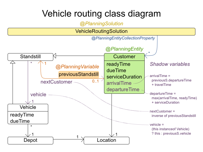
The vehicle routing with timewindows domain model makes heavily use of the shadow variable feature. This allows it to express its constraints more naturally, because properties such as arrivalTime and departureTime, are directly available on the domain model.
Road Distances Instead of Air Distances
In the real world, vehicles cannot follow a straight line from location to location: they have to use roads and highways. From a business point of view, this matters a lot:

For the optimization algorithm, this does not matter much, as long as the distance between two points can be looked up (and are preferably precalculated). The road cost does not even need to be a distance, it can also be travel time, fuel cost, or a weighted function of those. There are several technologies available to precalculate road costs, such as GraphHopper (embeddable, offline Java engine), Open MapQuest (web service) and Google Maps Client API (web service).

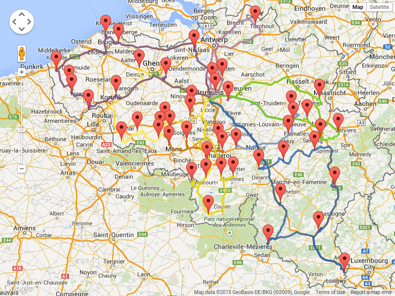
There are also several technologies to render it, such as Leaflet and Google Maps for developers: the optaplanner-webexamples-*.war has an example which demonstrates such rendering:

It is even possible to render the actual road routes with GraphHopper or Google Map Directions, but because of route overlaps on highways, it can become harder to see the standstill order:
Take special care that the road costs between two points use the same optimization criteria as the one used in Planner. For example, GraphHopper etc will by default return the fastest route, not the shortest route. Don’t use the km (or miles) distances of the fastest GPS routes to optimize the shortest trip in Planner: this leads to a suboptimal solution as shown below:

Contrary to popular belief, most users do not want the shortest route: they want the fastest route instead. They prefer highways over normal roads. They prefer normal roads over dirt roads. In the real world, the fastest and shortest route are rarely the same.
3.12. Project job scheduling
Schedule all jobs in time and execution mode to minimize project delays. Each job is part of a project. A job can be executed in different ways: each way is an execution mode that implies a different duration but also different resource usages. This is a form of flexible job shop scheduling.

Hard constraints:
- Job precedence: a job can only start when all its predecessor jobs are finished.
Resource capacity: do not use more resources than available.
- Resources are local (shared between jobs of the same project) or global (shared between all jobs)
- Resource are renewable (capacity available per day) or nonrenewable (capacity available for all days)
Medium constraints:
- Total project delay: minimize the duration (makespan) of each project.
Soft constraints:
- Total makespan: minimize the duration of the whole multi-project schedule.
The problem is defined by the MISTA 2013 challenge.
Problem size
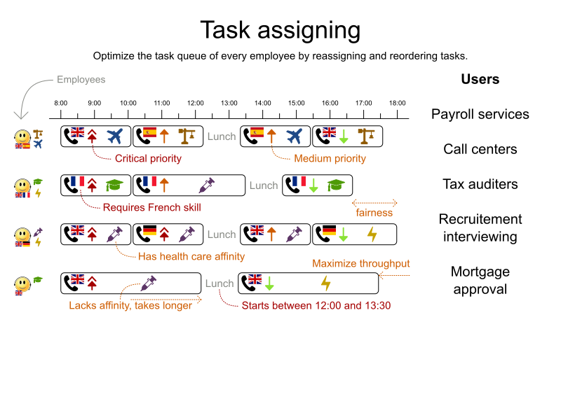
3.13. Task assigning
Assign each task to a spot in an employee’s queue. Each task has a duration which is affected by the employee’s affinity level with the task’s customer.
Hard constraints:
- Skill: Each task requires one or more skills. The employee must posses all these skills.
Soft level 0 constraints:
- Critical tasks: Complete critical tasks first, sooner than major and minor tasks.
Soft level 1 constraints:
Minimize makespan: Reduce the time to complete all tasks.
- Start with the longest working employee first, then the second longest working employee and so forth, to create fairness and load balancing.
Soft level 2 constraints:
- Major tasks: Complete major tasks as soon as possible, sooner than minor tasks.
Soft level 3 constraints:
- Minor tasks: Complete minor tasks as soon as possible.
Figure 3.9. Value proposition
Problem size
24tasks-8employees   has  24 tasks, 6 skills,  8 employees,   4 task types and  4 customers with a search space of   10^30.
50tasks-5employees   has  50 tasks, 5 skills,  5 employees,  10 task types and 10 customers with a search space of   10^69.
100tasks-5employees  has 100 tasks, 5 skills,  5 employees,  20 task types and 15 customers with a search space of  10^164.
500tasks-20employees has 500 tasks, 6 skills, 20 employees, 100 task types and 60 customers with a search space of 10^1168.
24tasks-8employees   has  24 tasks, 6 skills,  8 employees,   4 task types and  4 customers with a search space of   10^30.
50tasks-5employees   has  50 tasks, 5 skills,  5 employees,  10 task types and 10 customers with a search space of   10^69.
100tasks-5employees  has 100 tasks, 5 skills,  5 employees,  20 task types and 15 customers with a search space of  10^164.
500tasks-20employees has 500 tasks, 6 skills, 20 employees, 100 task types and 60 customers with a search space of 10^1168.Figure 3.10. Domain model

3.14. Exam timetabling (ITC 2007 track 1 - Examination)
Schedule each exam into a period and into a room. Multiple exams can share the same room during the same period.

Hard constraints:
- Exam conflict: Two exams that share students must not occur in the same period.
- Room capacity: A room’s seating capacity must suffice at all times.
- Period duration: A period’s duration must suffice for all of its exams.
Period related hard constraints (specified per dataset):
- Coincidence: Two specified exams must use the same period (but possibly another room).
- Exclusion: Two specified exams must not use the same period.
- After: A specified exam must occur in a period after another specified exam’s period.
Room related hard constraints (specified per dataset):
- Exclusive: One specified exam should not have to share its room with any other exam.
Soft constraints (each of which has a parametrized penalty):
- The same student should not have two exams in a row.
- The same student should not have two exams on the same day.
- Period spread: Two exams that share students should be a number of periods apart.
- Mixed durations: Two exams that share a room should not have different durations.
- Front load: Large exams should be scheduled earlier in the schedule.
- Period penalty (specified per dataset): Some periods have a penalty when used.
- Room penalty (specified per dataset): Some rooms have a penalty when used.
It uses large test data sets of real-life universities.
The problem is defined by the International Timetabling Competition 2007 track 1. Geoffrey De Smet finished 4th in that competition with a very early version of Planner. Many improvements have been made since then.
Problem Size
3.14.1. Domain model for Exam timetabling
The following diagram shows the main examination domain classes:
Figure 3.11. Examination domain class diagram

Notice that we’ve split up the exam concept into an Exam class and a Topic class. The Exam instances change during solving (this is the planning entity class), when their period or room property changes. The Topic, Period and Room instances never change during solving (these are problem facts, just like some other classes).
3.15. Nurse rostering (INRC 2010)
For each shift, assign a nurse to work that shift.

Hard constraints:
- No unassigned shifts (built-in): Every shift need to be assigned to an employee.
- Shift conflict: An employee can have only one shift per day.
Soft constraints:
Contract obligations. The business frequently violates these, so they decided to define these as soft constraints instead of hard constraints.
- Minimum and maximum assignments: Each employee needs to work more than x shifts and less than y shifts (depending on their contract).
- Minimum and maximum consecutive working days: Each employee needs to work between x and y days in a row (depending on their contract).
- Minimum and maximum consecutive free days: Each employee needs to be free between x and y days in a row (depending on their contract).
- Minimum and maximum consecutive working weekends: Each employee needs to work between x and y weekends in a row (depending on their contract).
- Complete weekends: Each employee needs to work every day in a weekend or not at all.
- Identical shift types during weekend: Each weekend shift for the same weekend of the same employee must be the same shift type.
- Unwanted patterns: A combination of unwanted shift types in a row. For example: a late shift followed by an early shift followed by a late shift.
Employee wishes:
- Day on request: An employee wants to work on a specific day.
- Day off request: An employee does not want to work on a specific day.
- Shift on request: An employee wants to be assigned to a specific shift.
- Shift off request: An employee does not want to be assigned to a specific shift.
- Alternative skill: An employee assigned to a skill should have a proficiency in every skill required by that shift.
The problem is defined by the International Nurse Rostering Competition 2010.
Figure 3.12. Value proposition

Problem size
There are three dataset types:
- sprint: must be solved in seconds.
- medium: must be solved in minutes.
- long: must be solved in hours.
Figure 3.13. Domain model

3.16. Traveling tournament problem (TTP)
Schedule matches between n teams.

Hard constraints:
- Each team plays twice against every other team: once home and once away.
- Each team has exactly one match on each timeslot.
- No team must have more than three consecutive home or three consecutive away matches.
- No repeaters: no two consecutive matches of the same two opposing teams.
Soft constraints:
- Minimize the total distance traveled by all teams.
The problem is defined on Michael Trick’s website (which contains the world records too).
Problem size
3.17. Cheap time scheduling
Schedule all tasks in time and on a machine to minimize power cost. Power prices differs in time. This is a form of job shop scheduling.
Hard constraints:
- Start time limits: Each task must start between its earliest start and latest start limit.
- Maximum capacity: The maximum capacity for each resource for each machine must not be exceeded.
- Startup and shutdown: Each machine must be active in the periods during which it has assigned tasks. Between tasks it is allowed to be idle to avoid startup and shutdown costs.
Medium constraints:
Power cost: Minimize the total power cost of the whole schedule.
- Machine power cost: Each active or idle machine consumes power, which infers a power cost (depending on the power price during that time).
- Task power cost: Each task consumes power too, which infers a power cost (depending on the power price during its time).
- Machine startup and shutdown cost: Every time a machine starts up or shuts down, an extra cost is inflicted.
Soft constraints (addendum to the original problem definition):
- Start early: Prefer starting a task sooner rather than later.
The problem is defined by the ICON challenge.
Problem size
3.18. Investment asset class allocation (Portfolio Optimization)
Decide the relative quantity to invest in each asset class.
Hard constraints:
Risk maximum: the total standard deviation must not be higher than the standard deviation maximum.
- Total standard deviation calculation takes asset class correlations into account by applying Markowitz Portfolio Theory.
- Region maximum: Each region has a quantity maximum.
- Sector maximum: Each sector has a quantity maximum.
Soft constraints:
- Maximize expected return.
Problem size
de_smet_1 has 1 regions, 3 sectors and 11 asset classes with a search space of 10^4.
irrinki_1 has 2 regions, 3 sectors and 6 asset classes with a search space of 10^3.
de_smet_1 has 1 regions, 3 sectors and 11 asset classes with a search space of 10^4.
irrinki_1 has 2 regions, 3 sectors and 6 asset classes with a search space of 10^3.Larger datasets have not been created or tested yet, but should not pose a problem. A good source of data is this Asset Correlation website.
3.19. Conference scheduling
Assign each conference talk to a timeslot and a room. Timeslots can overlap. Read/write to/from an *.xlsx file that can be edited with LibreOffice or Excel too.
Hard constraints:
- Talk type of timeslot: The type of a talk must match the timeslot’s talk type.
- Room unavailable timeslots: A talk’s room must be available during the talk’s timeslot.
- Room conflict: Two talks can’t use the same room during overlapping timeslots.
- Speaker unavailable timeslots: Every talk’s speaker must be available during the talk’s timeslot.
- Speaker conflict: Two talks can’t share a speaker during overlapping timeslots.
Generic purpose timeslot and room tags
- Speaker required timeslot tag: If a speaker has a required timeslot tag, then all his/her talks must be assigned to a timeslot with that tag.
- Speaker prohibited timeslot tag: If a speaker has a prohibited timeslot tag, then all his/her talks cannot be assigned to a timeslot with that tag.
- Talk required timeslot tag: If a talk has a required timeslot tag, then it must be assigned to a timeslot with that tag.
- Talk prohibited timeslot tag: If a talk has a prohibited timeslot tag, then it cannot be assigned to a timeslot with that tag.
- Speaker required room tag: If a speaker has a required room tag, then all his/her talks must be assigned to a room with that tag.
- Speaker prohibited room tag: If a speaker has a prohibited room tag, then all his/her talks cannot be assigned to a room with that tag.
- Talk required room tag: If a talk has a required room tag, then it must be assigned to a room with that tag.
- Talk prohibited room tag: If a talk has a prohibited room tag, then it cannot be assigned to a room with that tag.
- Talk mutually-exclusive-talks tag: Talks that share such a tag must not be scheduled in overlapping timeslots.
- Talk prerequisite talks: A talk must be scheduled after all its prerequisite talks.
Soft constraints:
- Theme track conflict: Minimize the number of talks that share a same theme tag during overlapping timeslots.
- Sector conflict: Minimize the number of talks that share a same sector tag during overlapping timeslots.
- Content audience level flow violation: For every content tag, schedule the introductory talks before the advanced talks.
- Audience level diversity: For every timeslot, maximize the number of talks with a different audience level.
- Language diversity: For every timeslot, maximize the number of talks with a different language.
Generic purpose timeslot and room tags
- Speaker preferred timeslot tag: If a speaker has a preferred timeslot tag, then all his/her talks should be assigned to a timeslot with that tag.
- Speaker undesired timeslot tag: If a speaker has a undesired timeslot tag, then all his/her talks should not be assigned to a timeslot with that tag.
- Talk preferred timeslot tag: If a talk has a preferred timeslot tag, then it should be assigned to a timeslot with that tag.
- Talk undesired timeslot tag: If a talk has a undesired timeslot tag, then it should not be assigned to a timeslot with that tag.
- Speaker preferred room tag: If a speaker has a preferred room tag, then all his/her talks should be assigned to a room with that tag.
- Speaker undesired room tag: If a speaker has a undesired room tag, then all his/her talks should not be assigned to a room with that tag.
- Talk preferred room tag: If a talk has a preferred room tag, then it should be assigned to a room with that tag.
- Talk undesired room tag: If a talk has a undesired room tag, then it should not be assigned to a room with that tag.
- Same day talks: All talks that share a same theme tag or content tag should be scheduled in the minimum number of days (ideally in the same day).
Figure 3.14. Value proposition

Problem size
18talks-6timeslots-5rooms    has  18 talks,  6 timeslots and  5 rooms with a search space of  10^26.
36talks-12timeslots-5rooms   has  36 talks, 12 timeslots and  5 rooms with a search space of  10^64.
72talks-12timeslots-10rooms  has  72 talks, 12 timeslots and 10 rooms with a search space of 10^149.
108talks-18timeslots-10rooms has 108 talks, 18 timeslots and 10 rooms with a search space of 10^243.
216talks-18timeslots-20rooms has 216 talks, 18 timeslots and 20 rooms with a search space of 10^552.
18talks-6timeslots-5rooms    has  18 talks,  6 timeslots and  5 rooms with a search space of  10^26.
36talks-12timeslots-5rooms   has  36 talks, 12 timeslots and  5 rooms with a search space of  10^64.
72talks-12timeslots-10rooms  has  72 talks, 12 timeslots and 10 rooms with a search space of 10^149.
108talks-18timeslots-10rooms has 108 talks, 18 timeslots and 10 rooms with a search space of 10^243.
216talks-18timeslots-20rooms has 216 talks, 18 timeslots and 20 rooms with a search space of 10^552.3.20. Rock tour
Drive the rock bus from show to show, but schedule shows only on available days.
Hard constraints:
- Schedule every required show.
- Schedule as many shows as possible.
Medium constraints:
- Maximize revenue opportunity.
- Minimize driving time.
- Visit sooner than later.
Soft constraints:
- Avoid long driving times.
Problem size
47shows has 47 shows with a search space of 10^59.
47shows has 47 shows with a search space of 10^59.3.21. Flight crew scheduling
Assign flights to pilots and flight attendants.
Hard constraints:
- Required skill: each flight assignment has a required skill. For example, flight AB0001 requires 2 pilots and 3 flight attendants.
- Flight conflict: each employee can only attend one flight at the same time
- Transfer between two flights: between two flights, an employee must be able to transfer from the arrival airport to the departure airport. For example, Ann arrives in Brussels at 10:00 and departs in Amsterdam at 15:00.
- Employee unavailability: the employee must be available on the day of the flight. For example, Ann is on PTO on 1-Feb.
Soft constraints:
- First assignment departing from home
- Last assignment arriving at home
- Load balance flight duration total per employee
Problem size
175flights-7days-Europe  has 2 skills, 50 airports, 150 employees, 175 flights and  875 flight assignments with a search space of  10^1904.
700flights-28days-Europe has 2 skills, 50 airports, 150 employees, 700 flights and 3500 flight assignments with a search space of  10^7616.
875flights-7days-Europe  has 2 skills, 50 airports, 750 employees, 875 flights and 4375 flight assignments with a search space of 10^12578.
175flights-7days-US      has 2 skills, 48 airports, 150 employees, 175 flights and  875 flight assignments with a search space of  10^1904.
175flights-7days-Europe  has 2 skills, 50 airports, 150 employees, 175 flights and  875 flight assignments with a search space of  10^1904.
700flights-28days-Europe has 2 skills, 50 airports, 150 employees, 700 flights and 3500 flight assignments with a search space of  10^7616.
875flights-7days-Europe  has 2 skills, 50 airports, 750 employees, 875 flights and 4375 flight assignments with a search space of 10^12578.
175flights-7days-US has 2 skills, 48 airports, 150 employees, 175 flights and 875 flight assignments with a search space of 10^1904.Appendix A. Versioning information
Documentation last updated on Friday, May 22, 2020.